What Is a Depreciation Schedule?
The reduction in the value of an asset over multiple years is called Depreciation. A Depreciation Schedule represents the reduction in the asset value or amount over its lifetime. This schedule is used for calculating total yearly depreciation.
Depreciation Terms:
- Cost (C): This is the cost of the asset.
- Salvage Value (Sn): This is the value of the asset at the end of the depreciation period.
- Depreciation Period (n) or Recovery Period: This is the useful life period of the asset.
How to Create a Monthly Depreciation Schedule in Excel: 8 Quick Steps
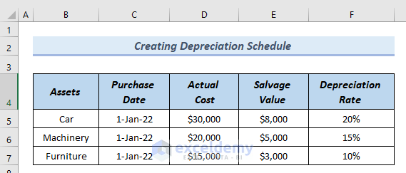
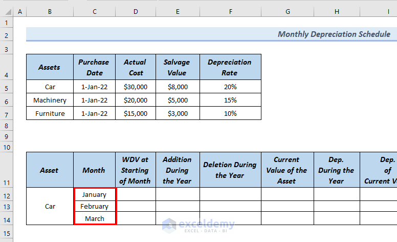
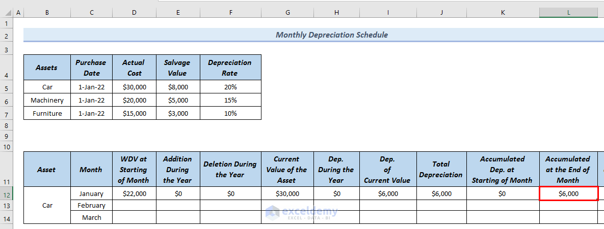
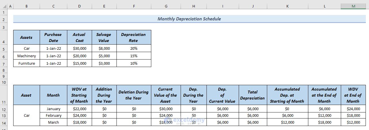
In the following dataset, you can see the Assets, Purchase Date, Actual Cost, Salvage Value, and Depreciations Rate columns.
Step 1 – Using the Data Validation Tool to Insert Assets in Excel
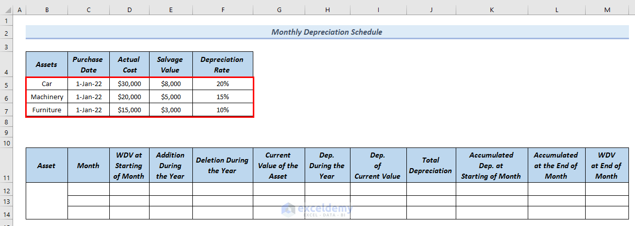
You can see the outline of the monthly Depreciation schedule with all the necessary terms. We want to insert only one asset name at a time and see the monthly depreciation schedule of that particular asset.
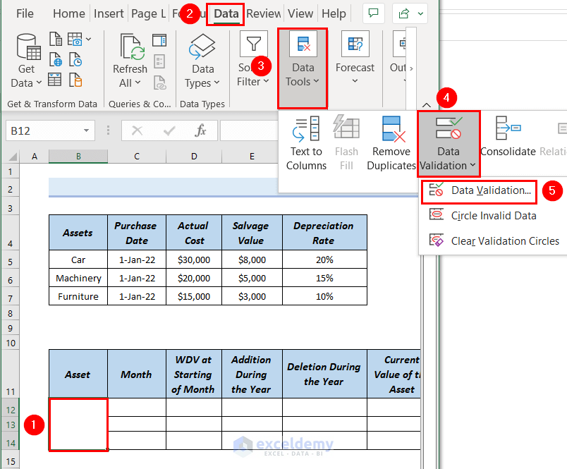
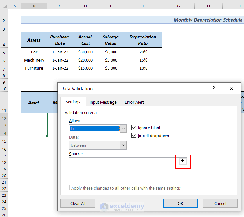
- Select merged cells B12:B14 and go to the Data tab.
- From Data Tools, select the Data Validation group.
- Select Data Validation.
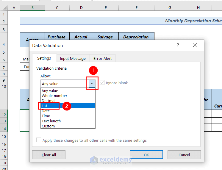
- A Data Validation dialog box will appear.
- From the Allow group, select List.
- Click on the upward arrow of the Source box to select the source cells.
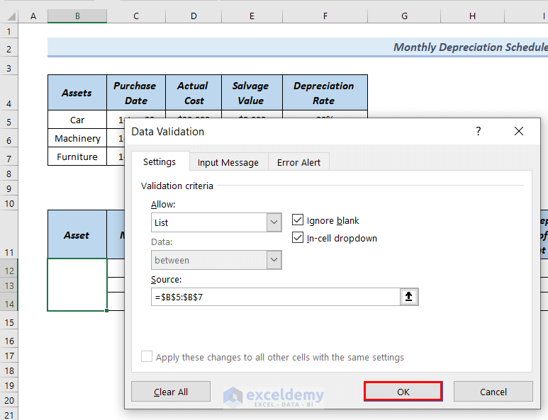
- Select cells B5:B7 as the Source cells.
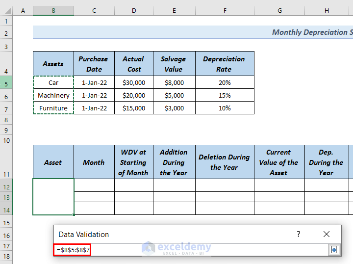
- Click OK in the Data Validation dialog box.
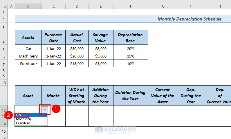
- Click on the drop-down arrow of cell B12. This will bring out the asset names.
- Select Car.
- Insert the months to show in the monthly depreciation schedule in cells C12:C14.
Read More: How to Create Depreciation Schedule in Excel
Step 2 – Calculating the Return Down Value at the Start of the Month
WDV indicates the return down value.
- Use the following formula in cell D12.
=IFS(B12=B5,D5-E5,B12=B6,D6-E6,B12=B7,D7-E7)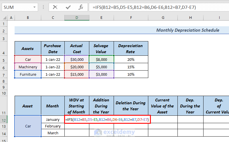
Formula Breakdown
- IFS(B12=B5,D5-E5,B12=B6,D6-E6,B12=B7,D7-E7) → the IFS function finds out whether one or more conditions are met, and then finds out the value of the corresponding True condition.
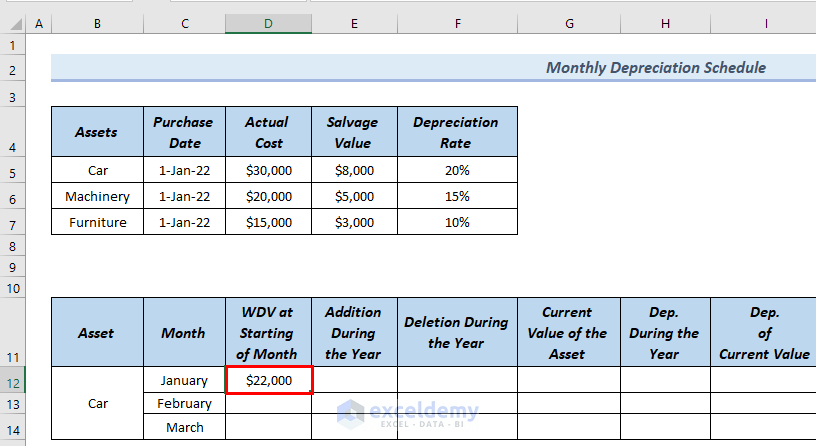
- IFS(B12=B5,D5-E5,B12=B6,D6-E6,B12=B7,D7-E7) → becomes output $22,000.
- Here, $22,000 is the WDV at Starting of Month of January.
- Press Enter.
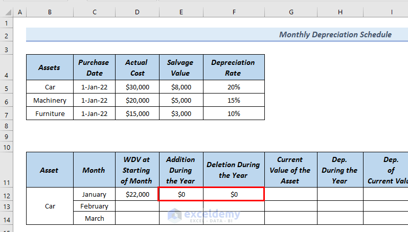
Since January is the starting month, there will be no Addition During the Year and Deletion During the Year.
- Put $0 in cells E12 and F12.
Step 3 – Evaluating the Current Value of Assets in the Depreciation Schedule
- Use the following formula in cell G12.
=IFS(B12=B5,D12+E12+E5-F12,B12=B6,D12+E12+E6-F12,B12=B7,D12+E12+E7-F12)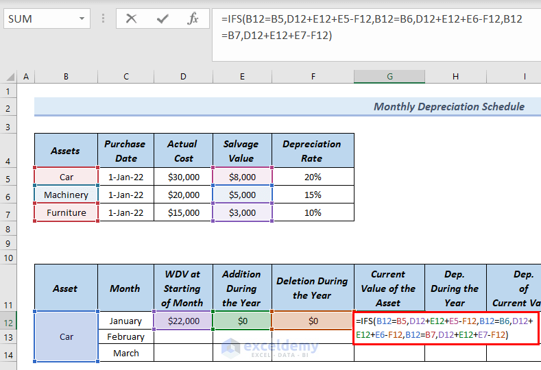
Formula Breakdown
- IFS(B12=B5,D12+E12+E5-F12,B12=B6,D12+E12+E6-F12,B12=B7,D12+E12+E7-F12)→ the IFS function finds out whether one or more conditions are met, and then finds out the value of the corresponding True condition.
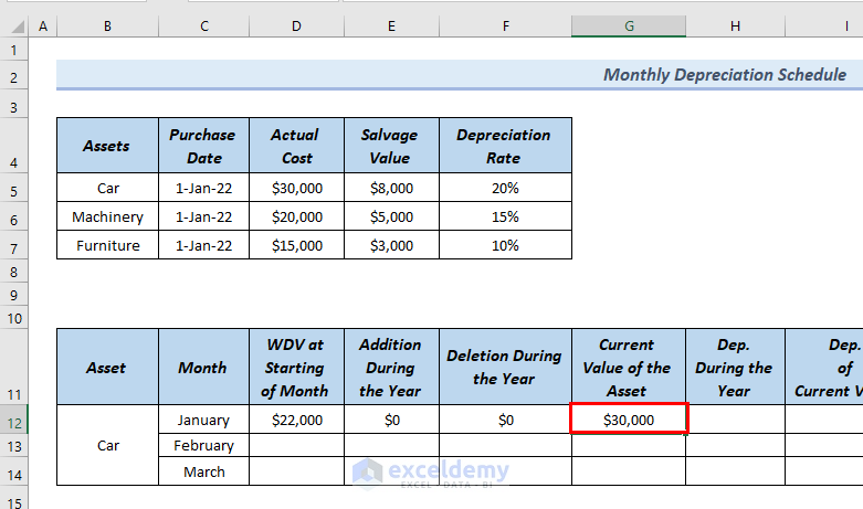
- IFS(B12=B5,D12+E12+E5-F12,B12=B6,D12+E12+E6-F12,B12=B7,D12+E12+E7-F12)→ becomes
- Output: $30,000
- Explanation: Here, $30,000 is the Current Value of Assets of month January.
- Press Enter.
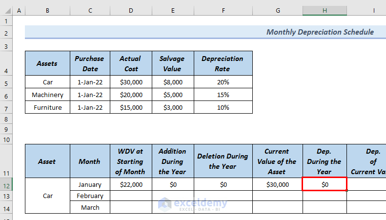
- Depreciation during the year is 0 for the starting month of January, so we put $0 in cell H12.
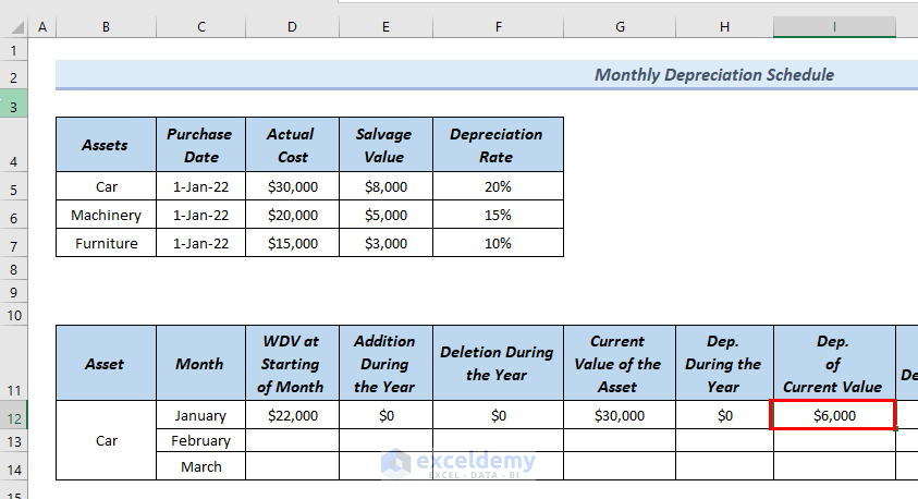
Step 4 – Calculating the Depreciation of Current Value for the First Month
- Use the following formula in cell I12.
=IFS(B12=B5,D5*F5,B12=B6,D6*F6,B12=B7,D7*F7)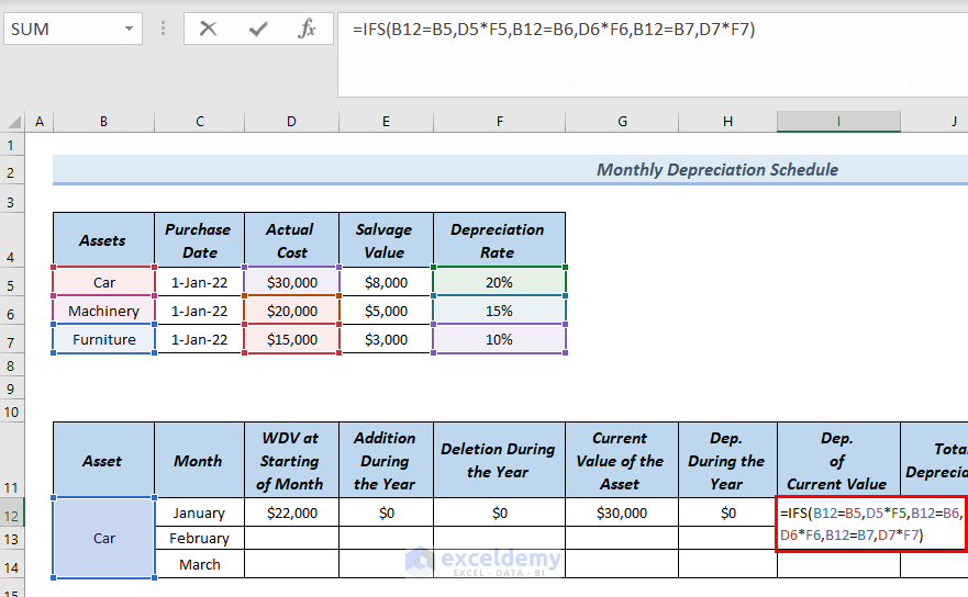
- Press Enter.
Read More: How to Create Vehicle Depreciation Calculator in Excel
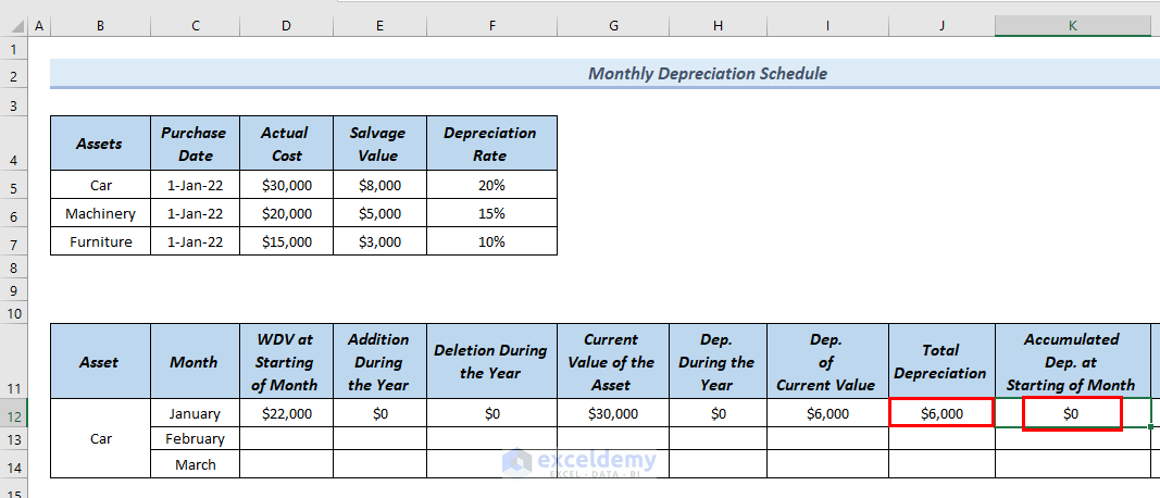
Step 5 – Computing the Total Depreciation in the Monthly Depreciation Schedule
- Use the following formula in cell J12.
=I12+H12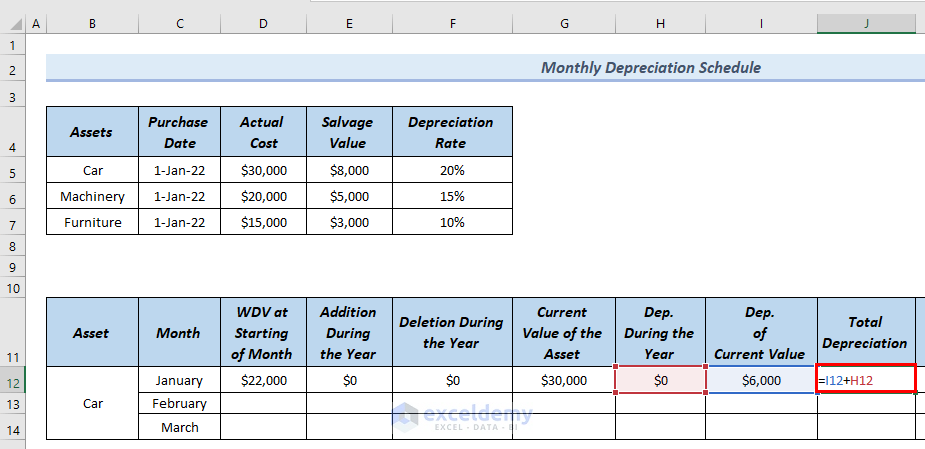
- Press Enter.
- Put $0 in cell K12 for calculating the value Accumulated Dep. at Starting of the Month.
Step 6 – Calculating Accumulated at the End of Month
- Use the following formula in cell L12.
=J12+K12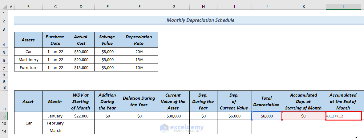
- Press Enter.
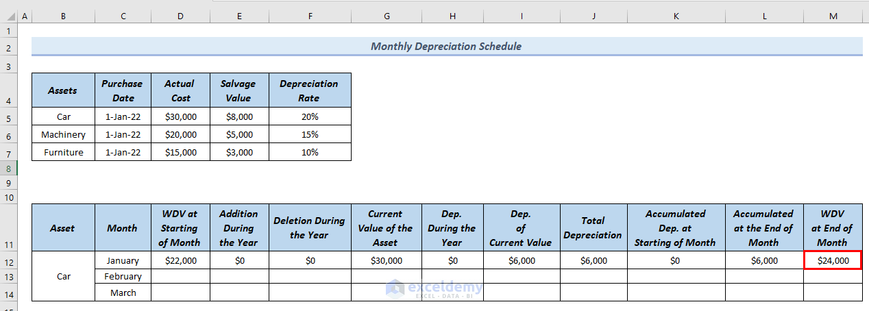
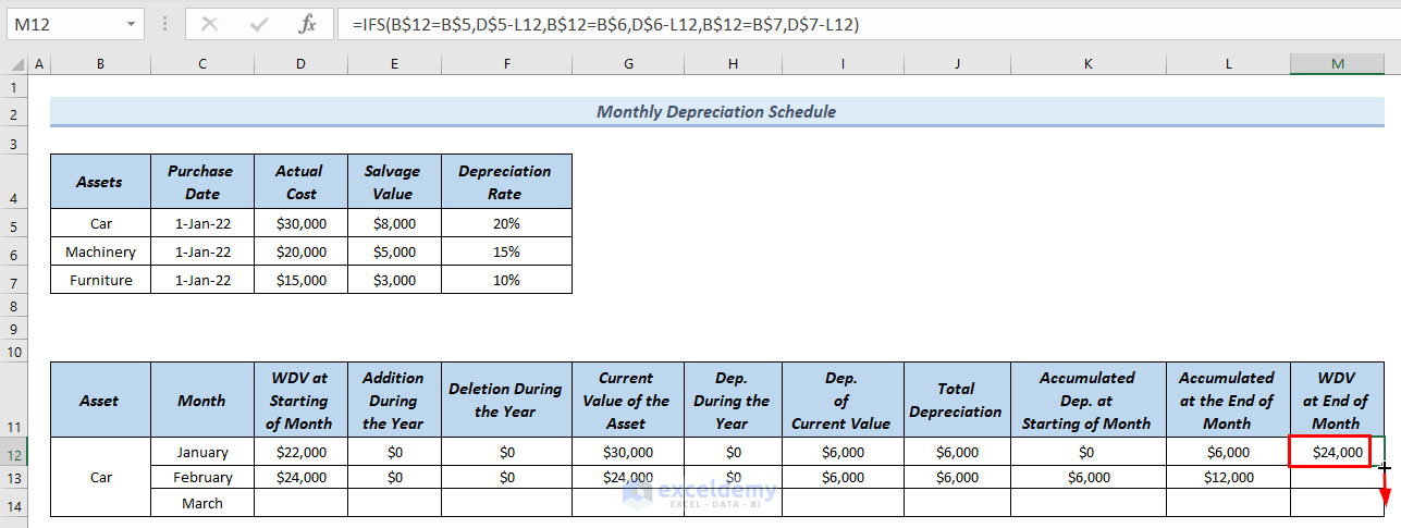
Step 7 – Evaluating the Return Down Value at End of Month
- Use the following formula in cell M12.
=IFS(B$12=B$5,D$5-L12,B$12=B$6,D$6-L12,B$12=B$7,D$7-L12)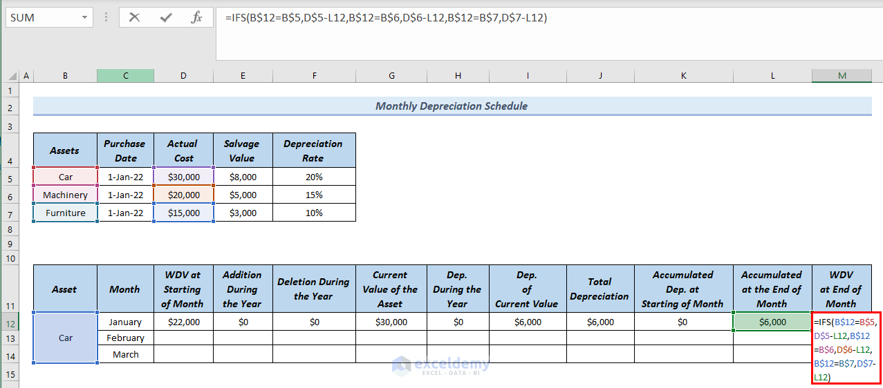
- Press Enter.
Step 8 – Creating a Depreciation Schedule for the Next Month
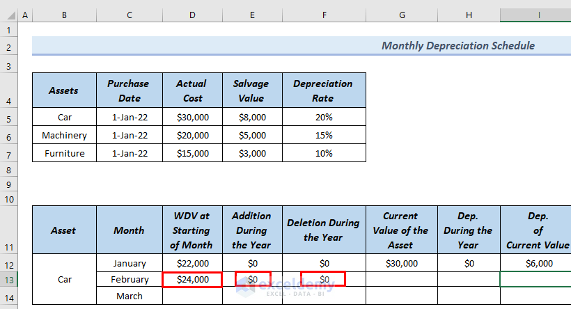
The return down value at starting of month February is equal to the return down value at the end of the month of January.
- In cell D13, use the following formula.
=M12This will input the value of cell M12 in cell D13.
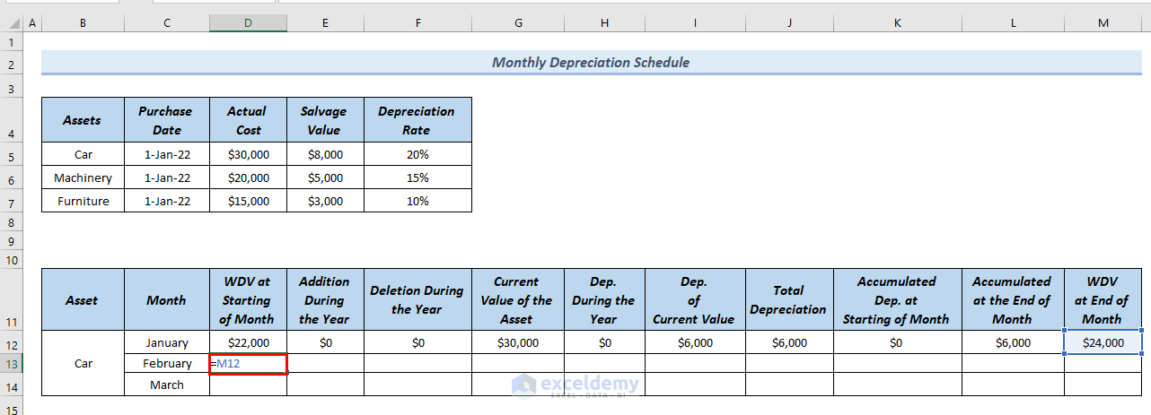
- Press Enter.
- Since Addition During the Year and Deletion During the Year are $0 for the month of February, put $0 in cells E13 and F13.
- Use the following formula in cell G13 to calculate the Current Value of Assets for the month of February.
=D13+E13-F13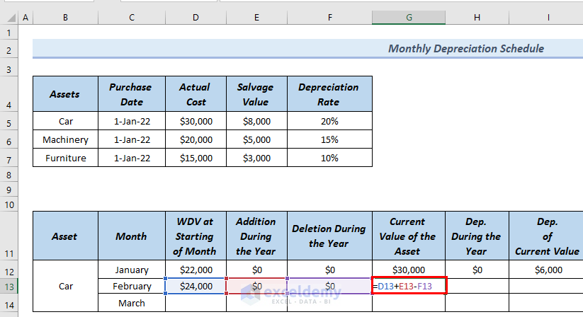
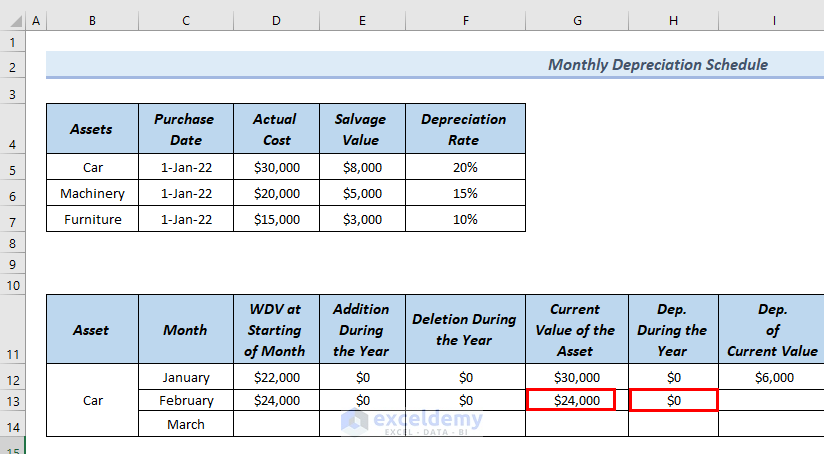
- Press Enter.
- Since Dep. During the Year is 0 for the month of February, put $0 in cell H13.
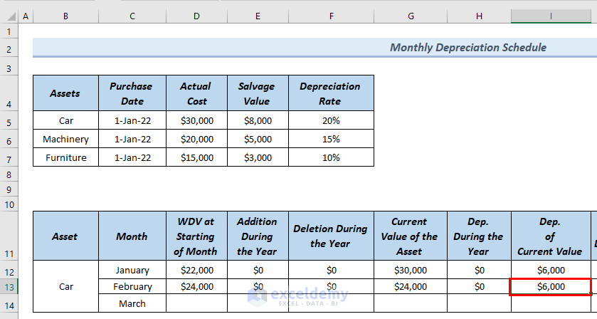
- Since the Dep. of Current Value is the same for the months of January and February, put the following formula in cell I13.
=I12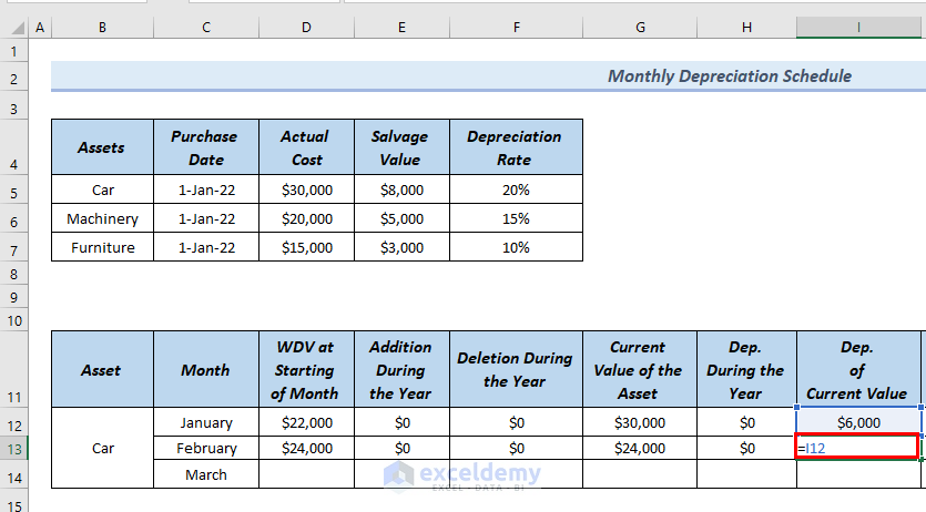
- Press Enter.
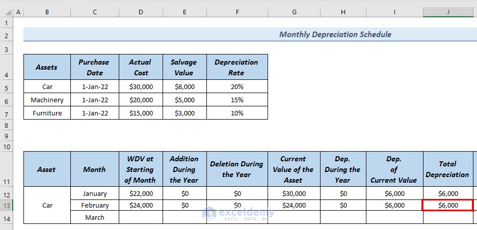
- Use the following formula in cell J13.
=I13+H13
- Press Enter.
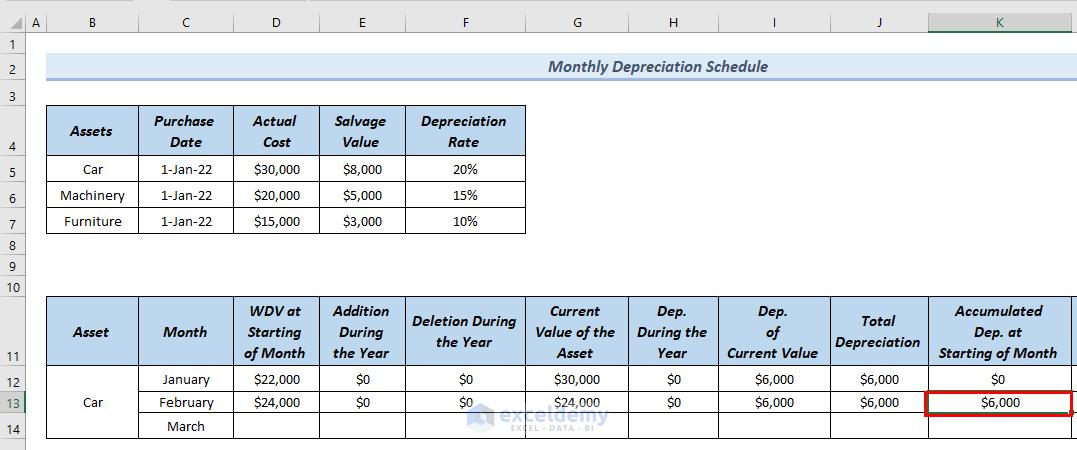
- Since the value of Accumulated Dep. of Starting of the Month for January and February is the same, use the following formula in cell K13.
=L12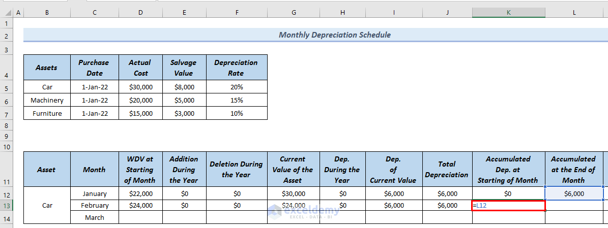
- Press Enter.
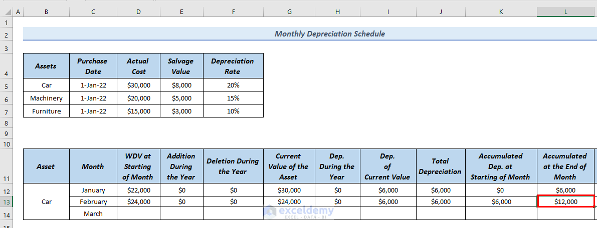
- Use the following formula in cell L13.
=J13+K13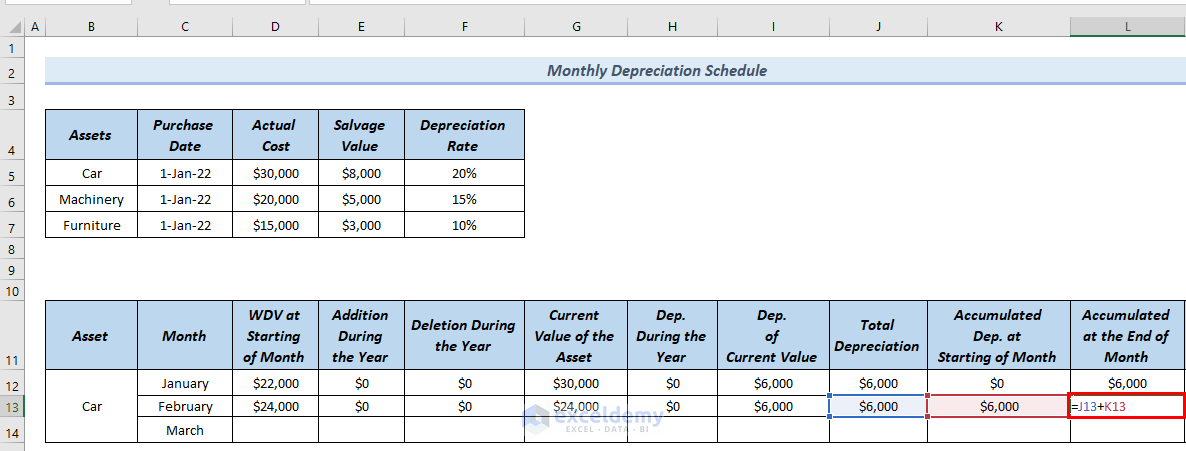
- Press Enter.
- To find out the WDV at the End of the Month for February, drag down the formula of cell M12 to cell M13 by the Fill Handle Tool.
- This completes the depreciation schedule for February.
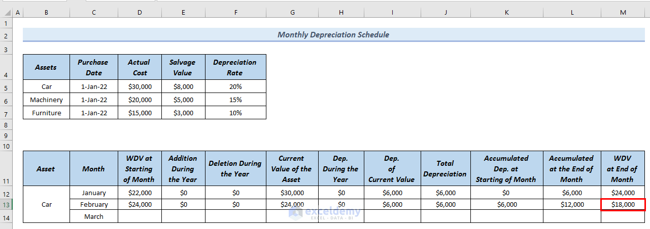
- Repeat the process to complete the March row of the depreciation schedule.
- You can see the complete monthly depreciation schedule for the asset Car.
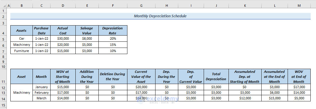
- You can see the complete monthly depreciation schedule for asset Machinery.
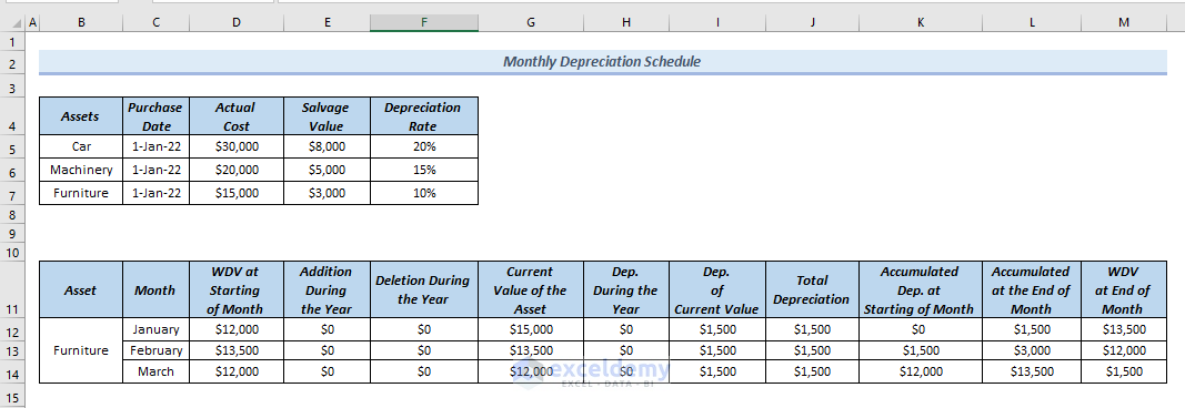
- You can see the complete monthly depreciation schedule for asset Furniture.
Read More: How to Create Rental Property Depreciation Calculator in Excel
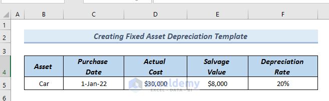
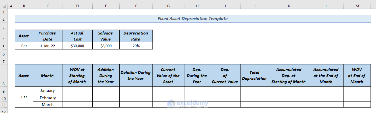
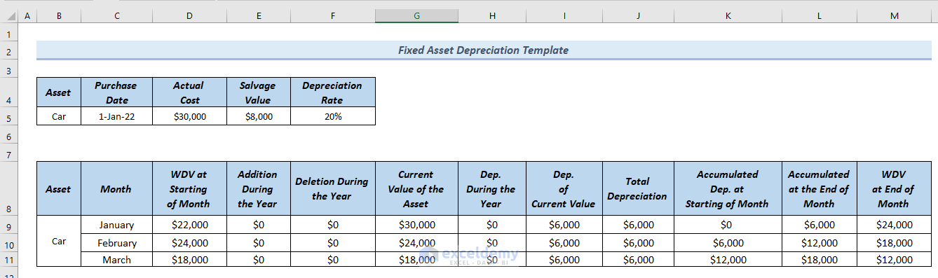
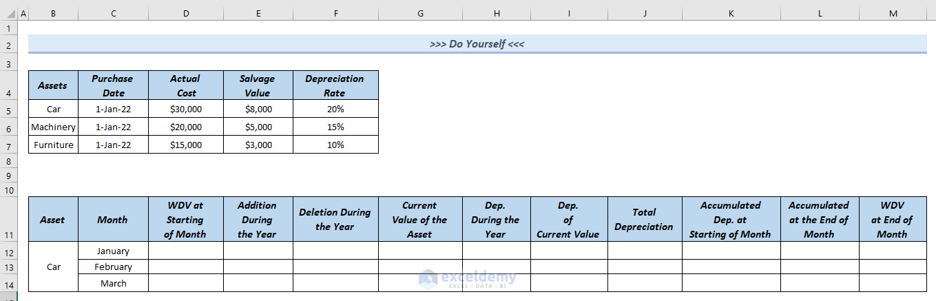
How to Create a Fixed Asset Depreciation Template in Excel
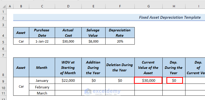
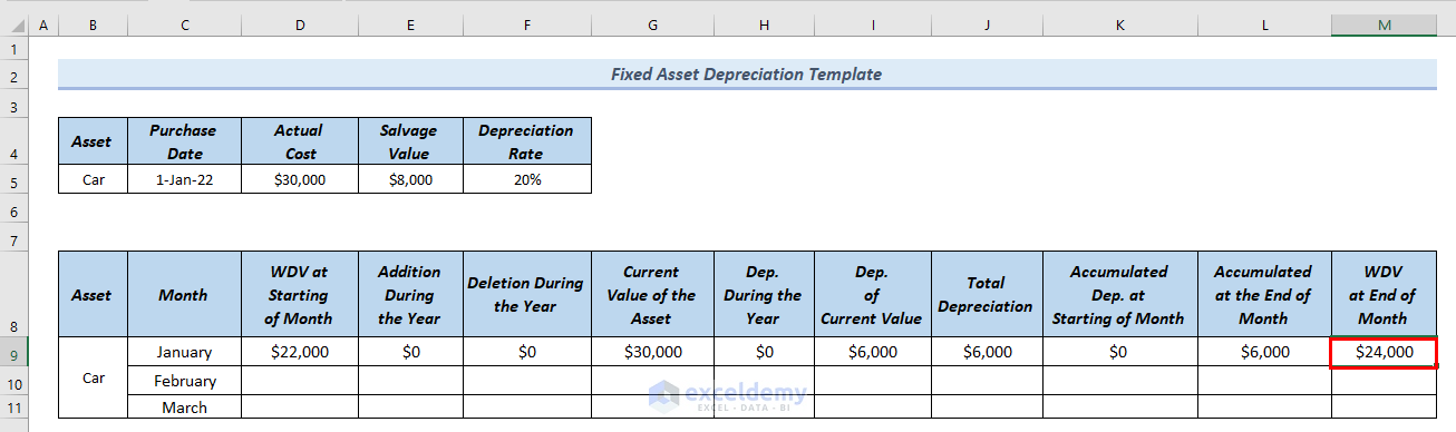
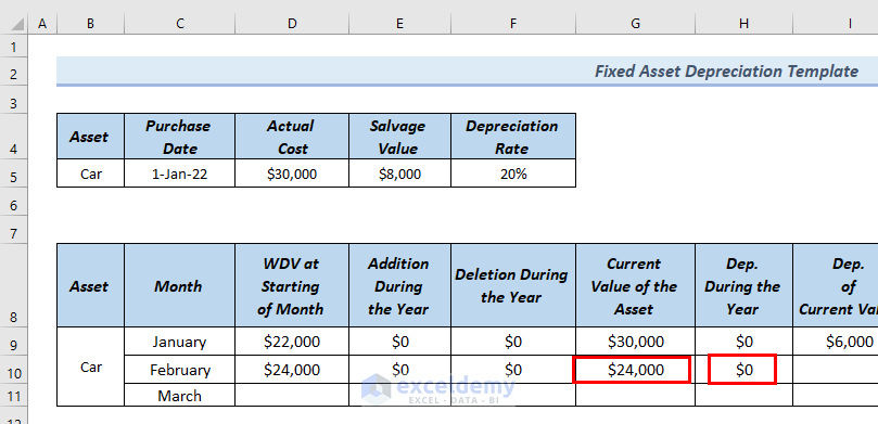
In the following table, you can see the properties of the asset Car.
- Here is the outline and months for the fixed asset depreciation template.
Step 1 – Calculating Depreciation for January
- Use the following formula in cell D9.
=D5-E5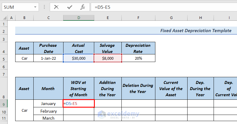
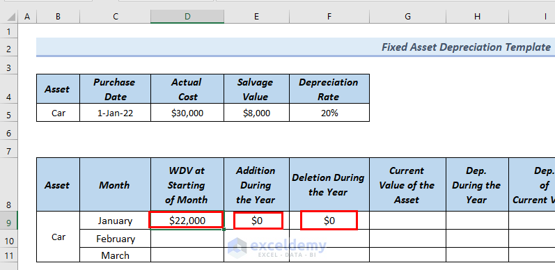
- Press Enter.
- Put $0 in cells E9 and F9.
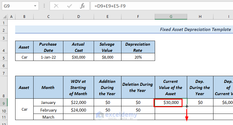
- Use the following formula in cell G9.
=IFS(B12=B5,D12+E12+E5-F12,B12=B6,D12+E12+E6-F12,B12=B7,D12+E12+E7-F12)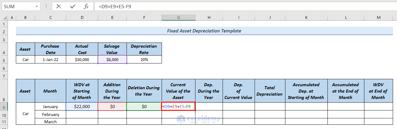
- Press Enter.
- Since the Dep. During the Year is $0 for the month of January, put $0 in cell H9.
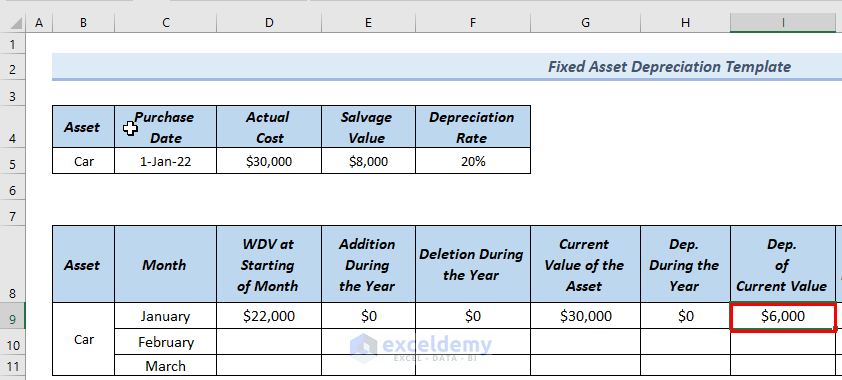
- Use the following formula in cell I9.
=D5*F5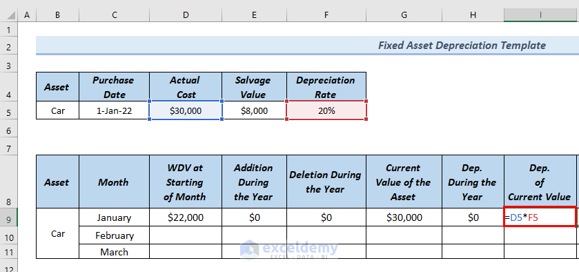
- Press Enter.
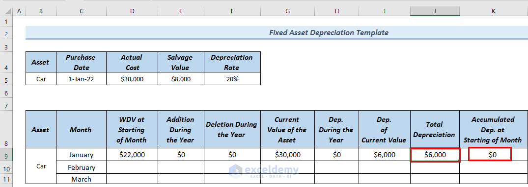
- Use the following formula in cell J9.
=I9+H9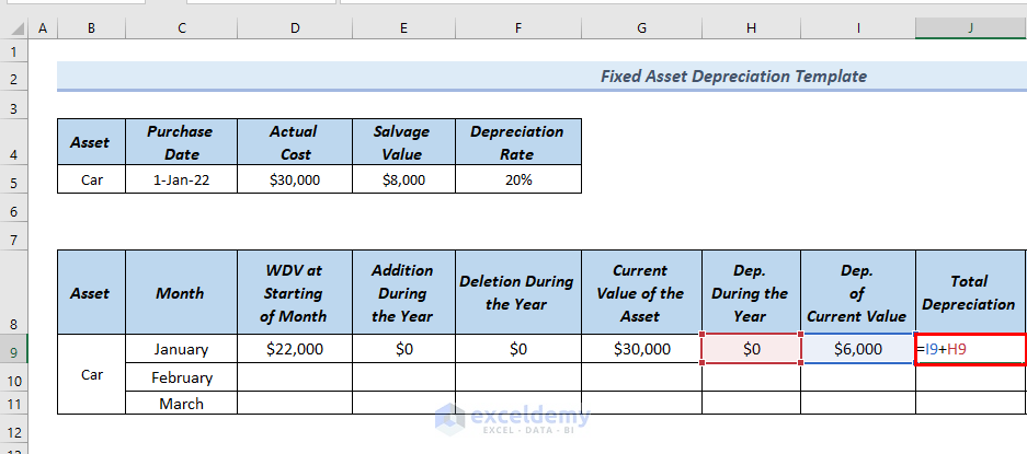
- Press Enter.
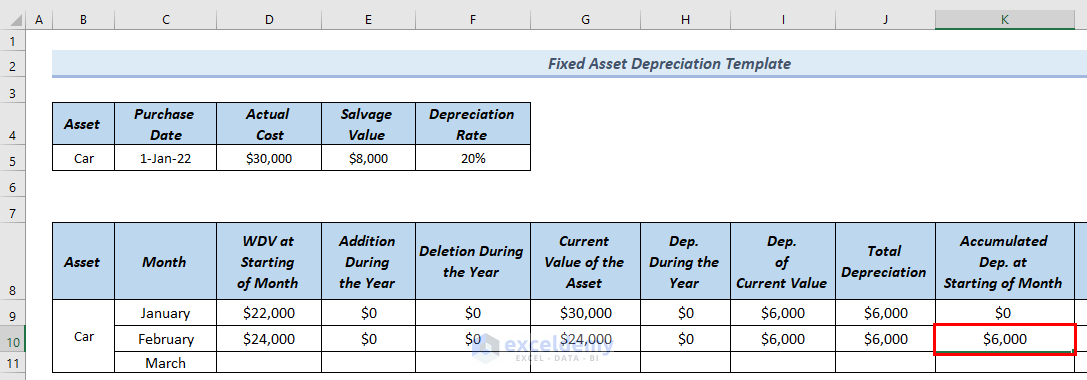
- Since Accumulated Dep. at Starting of Month is 0 for January, put $0 in cell K9.
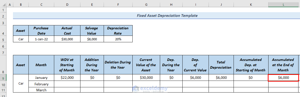
- Enter the following formula in cell L9.
=J9+K9 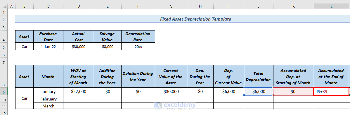
- Hit Enter.
- Use the following formula in cell M9.
=$D$5-L9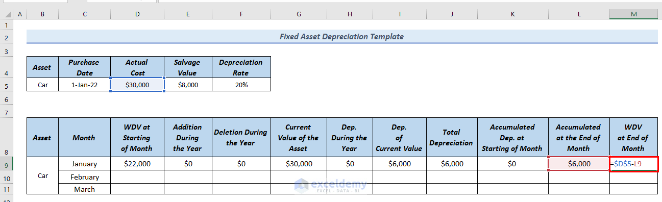
- Press Enter.
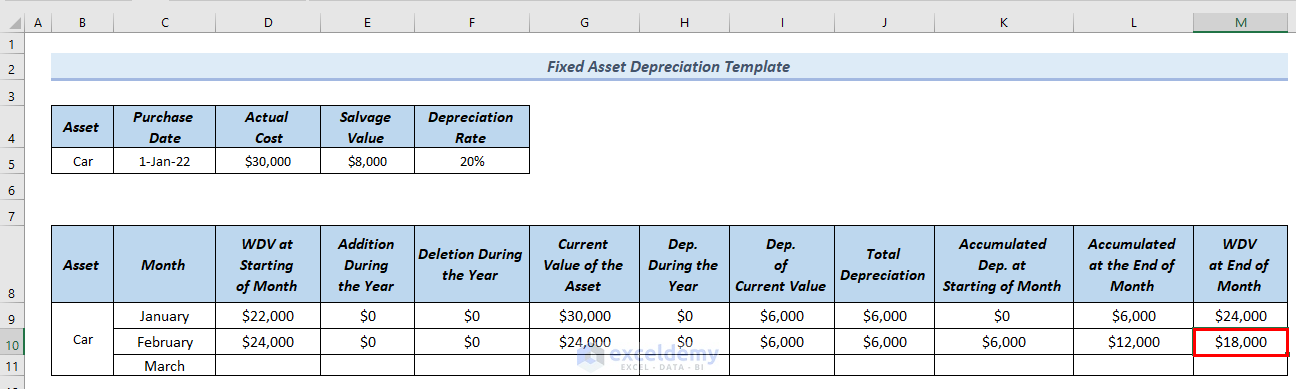
Step 2 – Creating a Depreciation Schedule for February
- Since WDV at End of the Month of January is equal to WDV at Starting of Month of February, in cell D13 use the following formula.
=M9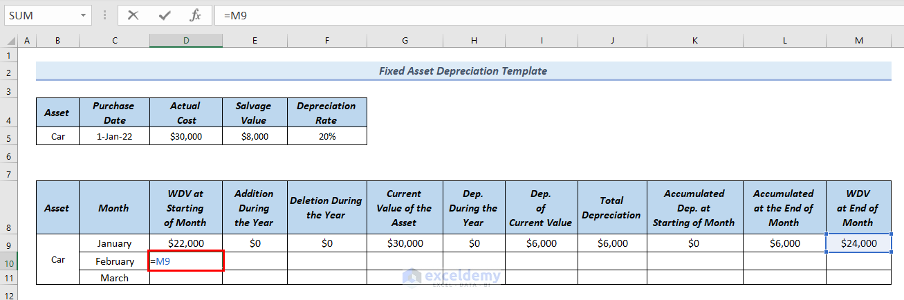
- Press Enter.
- Since the Addition During the Year and Deletion During the Year are $0 for the month of February, put $0 in cells E10 and F10.
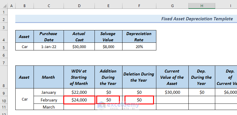
- To find out the Current Value of the Asset for the month of February, drag down the formula of cell G9 to cell G10 with a Fill Handle tool.
- Since Dep. During the Year for the month of February is 0, put $0 in cell H10.
- Since the value of Dep. of Current Value for January is equal to Dep. of Current Value in February, use the following formula in cell I10.
=I9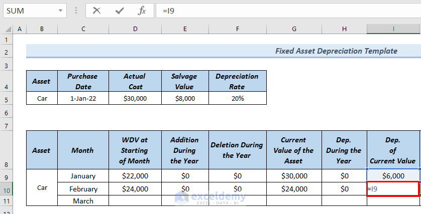
- Press Enter.
- Use the following formula in cell J10.
=I10+H10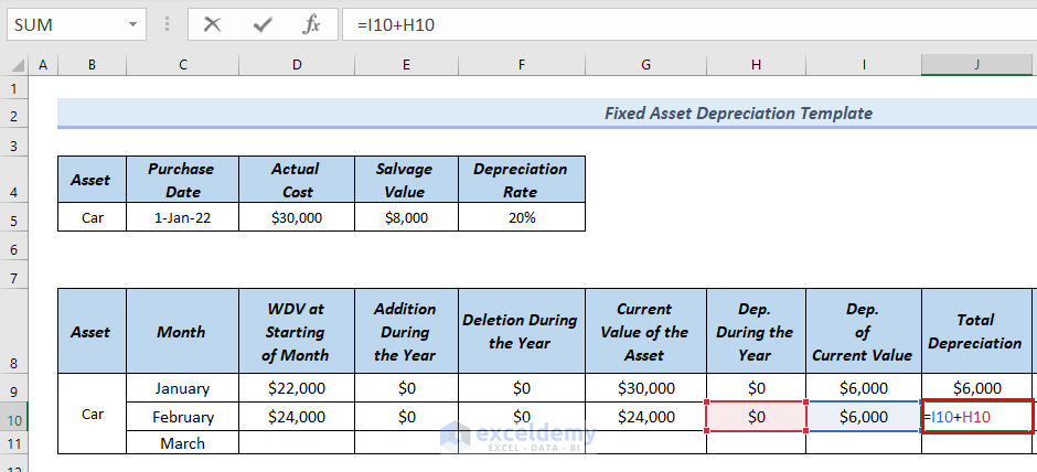
- Press Enter.
- Since the Accumulated Dep. at the start of the Months for January and February are equal, use the following formula in cell K10.
=L9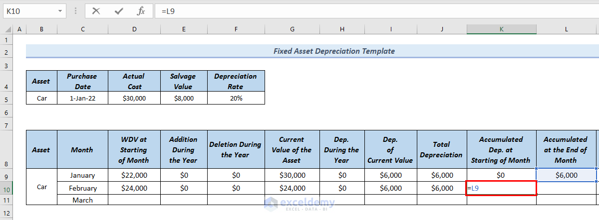
- Press Enter.
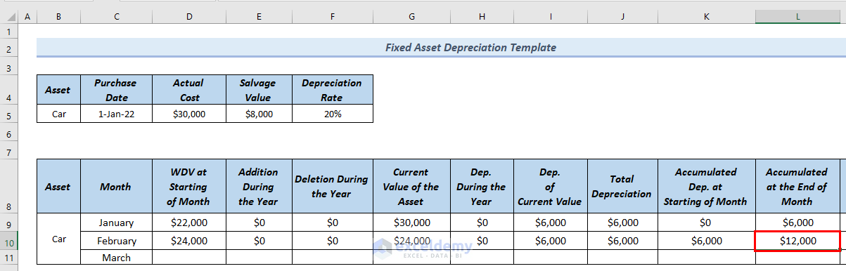
- Use the following formula in cell L10.
=J10+K10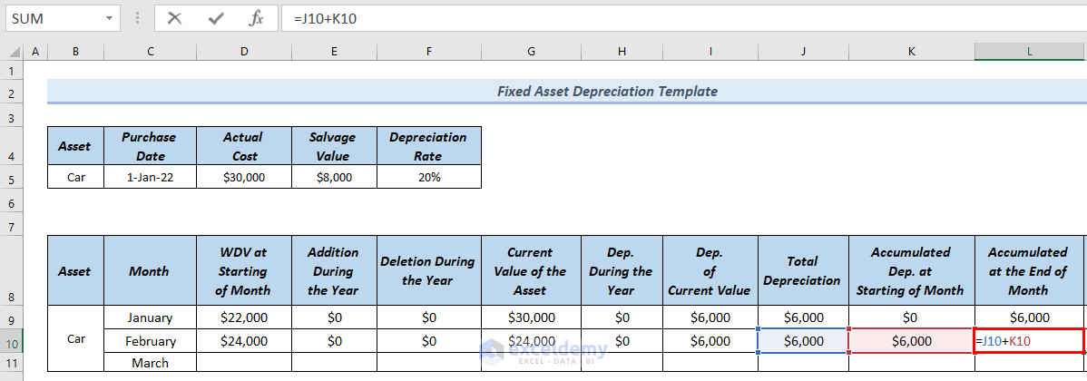
- Press Enter.
- Use the following formula in cell M10.
=$D$5-L10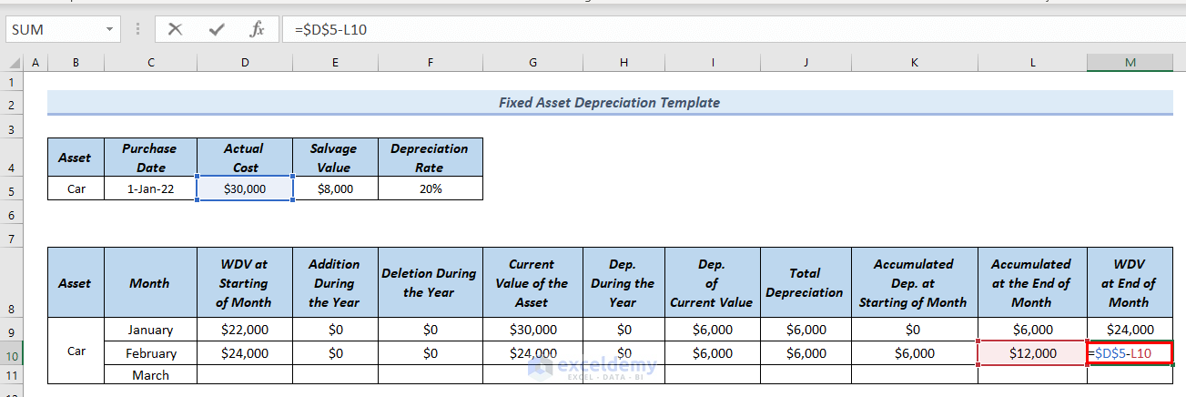
- Press Enter.
- Similarly, we created the depreciation schedule for the month of March.
Practice Section
You can download the Excel file to practice or use it as a template.
Download the Practice Workbook
<< Go Back to Depreciation Template | Finance Template | Excel Templates
Get FREE Advanced Excel Exercises with Solutions!

A Most Excellent Article !
Thank You
Aubrey Meissenheimer
Pretoria, South Africa
Dear Aubrey
You are most welcome. Your appreciation means a lot to us.
Regards
ExcelDemy