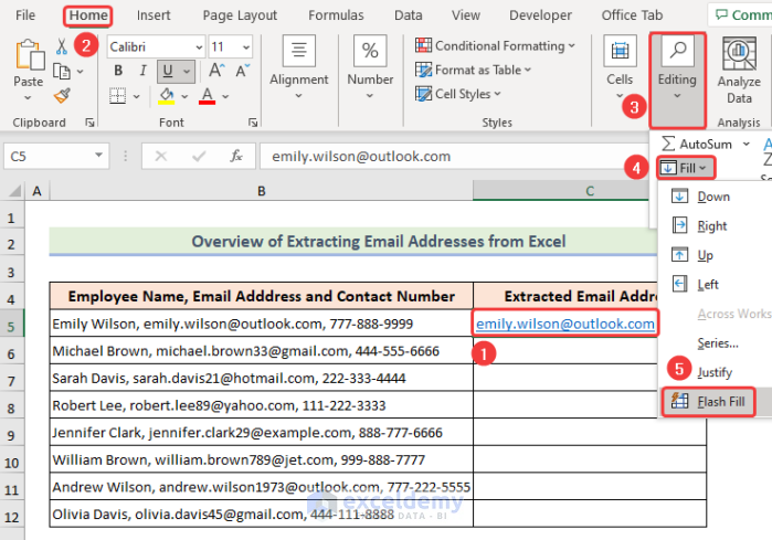
Here’s a dataset that will provide an overview of extracting email addresses from Excel. It contains addresses embedded into larger strings in cells.
How to Extract Email Addresses from Excel: 4 Ways
Method 1 – Extracting Email Addresses Using Excel Tools
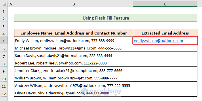
Case 1.1 – Using Flash Fill
- Type your desired content to the next column. We wrote the email address from B5 into cell C5.
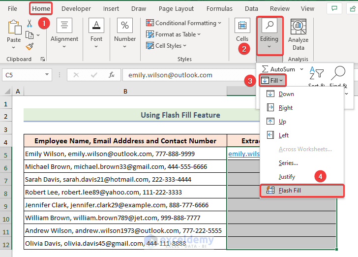
- Selecting cells C5:C12.
- Click Flash Fill from the Home ribbon (choose Editing, then Fill).
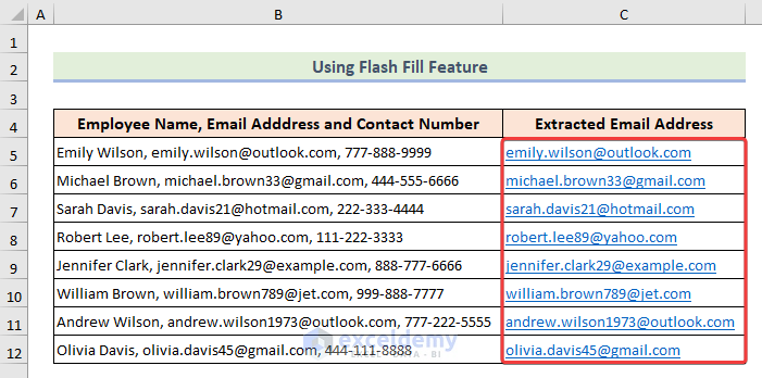
- You will get extracted email addresses in the table.
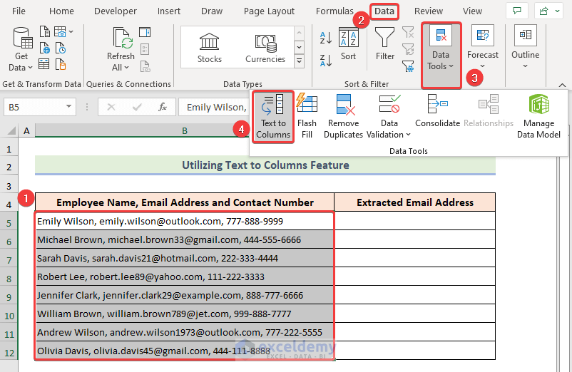
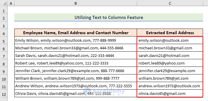
Case 1.2 – Utilizing the Text to Columns Feature
- Choose the table from which you want to extract email addresses.
- Click Text to Columns from the Data tab (option Data Tools).
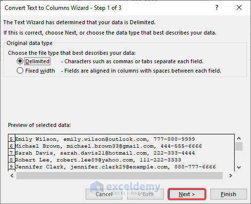
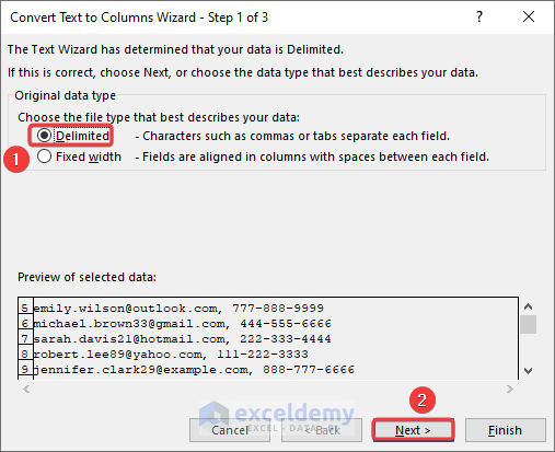
- From the Convert Text to Columns Wizard window, check Delimited and press Next.
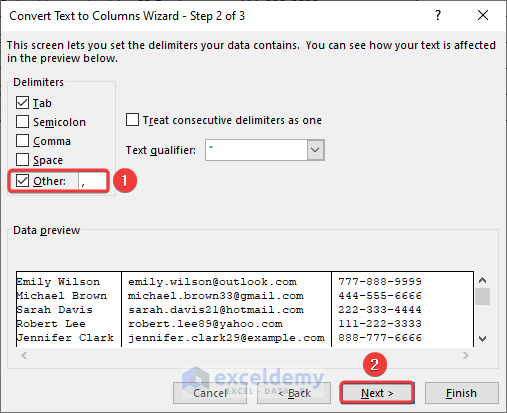
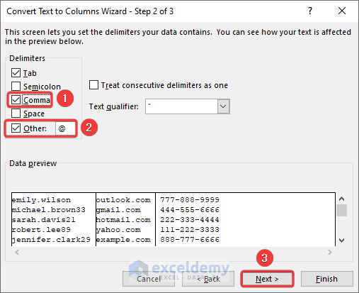
- Put a comma (,) into the Other section (or check Comma) and click Next.
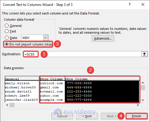
- Choose your destination cell (=$C$5), check the Do not import column option and click on the columns you don’t need in Data preview, then press Finish.
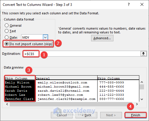
- This extracts email addresses from the cells.
Read More: How to Make an Address Book in Excel
Method 2 – Extracting Email Addresses from a Single Column
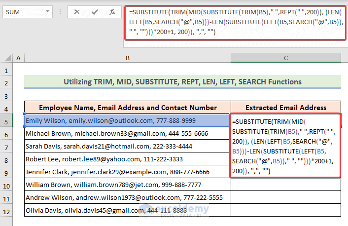
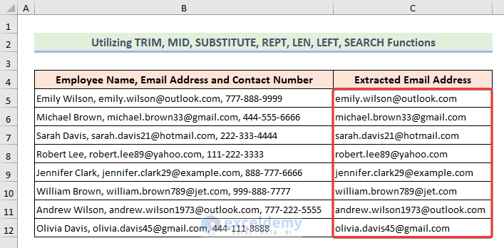
Case 2.1 – Utilizing TRIM, MID, SUBSTITUTE, REPT, LEN, LEFT, and SEARCH Functions
- Choose a cell (C5) and apply the following formula.
=SUBSTITUTE(TRIM(MID(SUBSTITUTE(TRIM(B5)," ",REPT(" ",200)), (LEN(LEFT(B5,SEARCH("@",B5)))-LEN(SUBSTITUTE(LEFT(B5,SEARCH("@",B5))," ", "")))*200+1, 200)), ",", "")Formula Breakdown
- LEFT(B5,SEARCH(“@”,B5)
This section finds the text from the beginning of cell (B5) up to the “@” symbol.
- SUBSTITUTE(LEFT(B5,SEARCH(“@”,B5)),” “, “”)
This section removes any spaces from the text obtained in step 1. It replaces each space (” “) with an empty string (“”).
- LEN(SUBSTITUTE(LEFT(B5,SEARCH(“@”,B5)),” “, “”))
This portion calculates the length of the text obtained in step 2 and counts the number of characters in the text.
- (LEN(LEFT(B5,SEARCH(“@”,B5)))-LEN(SUBSTITUTE(LEFT(B5,SEARCH(“@”,B5)),” “, “”)))
This step subtracts the length of the text without spaces from the length of the original text.
- REPT(” “,200)
REPT generates a string consisting of 200 spaces by repeating the space character (” “) 200 times.
- SUBSTITUTE(TRIM(B5),” “,REPT(” “,200))
This replaces each occurrence of a single space in cell (B5) with 200 spaces. Then, the TRIM function removes any leading or trailing spaces.
- MID(SUBSTITUTE(TRIM(B5),” “,REPT(” “,200)), (LEN(LEFT(B5,SEARCH(“@”,B5)))-LEN(SUBSTITUTE(LEFT(B5,SEARCH(“@”,B5)),” “, “”)))*200+1, 200)
This extracts a portion of the modified text obtained in step 6. Hence, it starts from a specific position and retrieves a substring of length 200.
- TRIM(MID(SUBSTITUTE(TRIM(B5),” “,REPT(” “,200)), (LEN(LEFT(B5,SEARCH(“@”,B5)))-LEN(SUBSTITUTE(LEFT(B5,SEARCH(“@”,B5)),” “, “”)))*200+1, 200)), “,”, “”)
This trims any leading or trailing spaces from the substring obtained in step 7.
- SUBSTITUTE(TRIM(MID(SUBSTITUTE(TRIM(B5),” “,REPT(” “,200)), (LEN(LEFT(B5,SEARCH(“@”,B5)))-LEN(SUBSTITUTE(LEFT(B5,SEARCH(“@”,B5)),” “, “”)))*200+1, 200)), “,”, “”)
This replaces any commas (“,”) in the trimmed substring with empty strings (“”).
- Hit the Enter key and drag the fill handle down to get the final output.
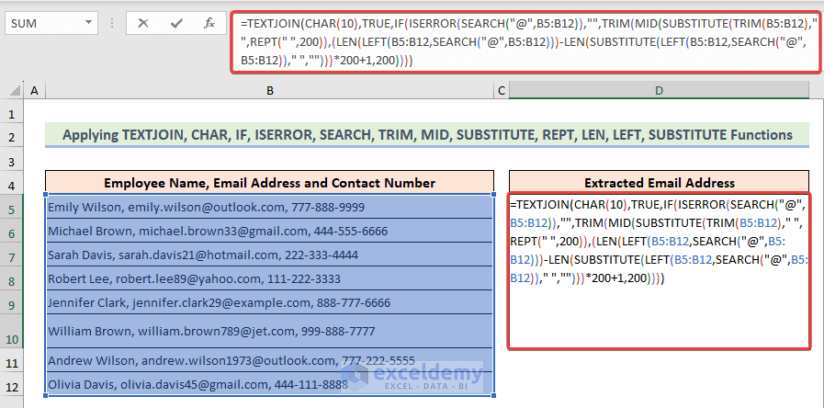
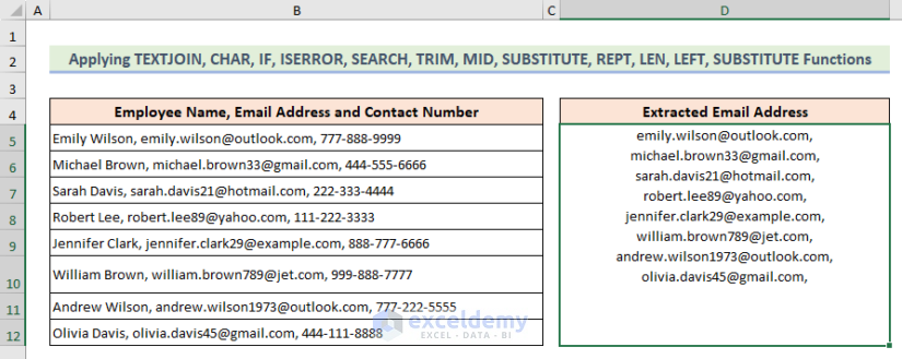
Case 2.2 – Applying TEXTJOIN, CHAR, IF, ISERROR, SEARCH, TRIM, MID, SUBSTITUTE, REPT, LEN, LEFT, and SUBSTITUTE Functions
- Select a cell (C5) and copy the following formula inside:
=TEXTJOIN(CHAR(10),TRUE,IF(ISERROR(SEARCH("@",B5:B12)),"",TRIM(MID(SUBSTITUTE(TRIM(B5:B12)," ",REPT(" ",200)),(LEN(LEFT(B5:B12,SEARCH("@",B5:B12)))-LEN(SUBSTITUTE(LEFT(B5:B12,SEARCH("@",B5:B12))," ","")))*200+1,200))))Formula Breakdown
- SEARCH(“@”,B5:B12)
Here the SEARCH function searches for the “@” symbol in cells (B5:B12) and returns an array of values, indicating the position of “@” in each cell.
- ISERROR(SEARCH(“@”,B5:B12))
This function checks if an error occurs in the search operation. It returns an array of TRUE or FALSE values, where TRUE represents an error and FALSE represents a successful search.
- IF(ISERROR(SEARCH(“@”,B5:B12)),””,TRIM(MID(SUBSTITUTE(TRIM(B5:B12),” “,REPT(” “,200)),(LEN(LEFT(B5:B12,SEARCH(“@”,B5:B12)))-LEN(SUBSTITUTE(LEFT(B5:B12,SEARCH(“@”,B5:B12)),” “,””)))*200+1,200))))
Here an IF statement checks the array from step 2. If an error is found, it returns an empty string (“”). Otherwise, it proceeds with the next part of the formula.
- LEFT(B5:B12,SEARCH(“@”,B5:B12))
This extracts the text from the beginning of each cell in the range B5 to B12 up to the “@” symbol.
- SUBSTITUTE(LEFT(B5:B12,SEARCH(“@”,B5:B12)),” “,””)
This removes any spaces from the text obtained in step 4. It replaces each space (” “) with an empty string (“”).
- LEN(SUBSTITUTE(LEFT(B5:B12,SEARCH(“@”,B5:B12)),” “,””))
This calculates the length of the text obtained in step 5 for each cell and returns an array of values representing the length.
- (LEN(LEFT(B5:B12,SEARCH(“@”,B5:B12)))-LEN(SUBSTITUTE(LEFT(B5:B12,SEARCH(“@”,B5:B12)),” “,””)))*200+1
This part calculates the starting position for the MID function. Then, it subtracts the length of the text without spaces from the length of the original text and multiplies the result by 200.
- REPT(” “,200)
This generates a string consisting of 200 spaces. After that, it repeats the space character (” “) 200 times.
- SUBSTITUTE(TRIM(B5:B12),” “,REPT(” “,200))
This replaces each occurrence of a single space in the original text (B5:B12) with 200 spaces. The TRIM function removes any leading or trailing spaces.
- MID(SUBSTITUTE(TRIM(B5:B12),” “,REPT(” “,200)),(LEN(LEFT(B5:B12,SEARCH(“@”,B5:B12)))-LEN(SUBSTITUTE(LEFT(B5:B12,SEARCH(“@”,B5:B12)),” “,””)))*200+1,200)
This extracts a portion of the modified text obtained in step 9. It starts from the position calculated in step 7 and retrieves a substring of length 200 for each cell.
- TEXTJOIN(CHAR(10),TRUE,IF(ISERROR(SEARCH(“@”,B5:B12)),””,TRIM(MID(SUBSTITUTE(TRIM(B5:B12),” “,REPT(” “,200)),(LEN(LEFT(B5:B12,SEARCH(“@”,B5:B12)))-LEN(SUBSTITUTE(LEFT(B5:B12,SEARCH(“@”,B5:B12)),” “,””)))*200+1,200))))
This function concatenates the array of trimmed substrings obtained in step 11 into a single text string, separated by a line break (CHAR(10)). The TRUE argument indicates that empty values should be ignored.
- Hit Enter and drag the Fill Handle down to fill the column.
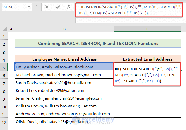
Case 2.3 – Combining SEARCH, ISERROR, IF and TEXTJOIN Functions
- Choose a cell (C5), copy the following formula into it, hit Enter, and drag the FIll handle down:
=IF(ISERROR(SEARCH("@", B5)), "", MID(B5, SEARCH(",", B5) + 2, LEN(B5) - SEARCH(",", B5) - 1))Formula Breakdown
- ISERROR(SEARCH(“@”, B5))
The SEARCH function searches for the “@” symbol in cell (B5) and returns the position of “@” in the text. The ISERROR function checks if an error occurs in the search operation.
- IF(ISERROR(SEARCH(“@”, B5)), “”, …)
This is an IF statement that checks if an error occurs. If an error is found it returns an empty string (“”).
- MID(B5, SEARCH(“,”, B5) + 2, LEN(B5) – SEARCH(“,”, B5) – 1)
Finally, the extraction of a portion of the text in cell (B5) happens. Then, it starts from the position calculated in step 2 and retrieves a substring of length obtained.
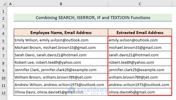
- We have the extracted the email addresses.
Read More: How to Format a Column for Email Addresses in Excel
Method 3 – Extracting Email Addresses from Multiple Columns
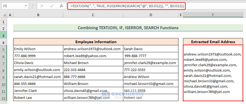
Case 3.1 – Using TEXTJOIN, IF, ISERROR, and SEARCH Functions Together
- Choose a cell (F5), copy the below formula, and hit Enter to get the output.
=TEXTJOIN(", ", TRUE, IF(ISERROR(SEARCH("@", B5:D12)), "", B5:D12))Formula Breakdown
- ISERROR(SEARCH(“@”, B5:D12))
The SEARCH function searches for the “@” symbol in cells (B5:D12) and returns the position of “@” in the text. The ISERROR function checks if an error occurs in the search operation.
- IF(ISERROR(SEARCH(“@”, B5:D12)), “”, B5:D12)
Here the IF statement checks if an error is found and returns an empty string (“”). Otherwise, it returns the corresponding cell value from the cells (B5:D12).
- TEXTJOIN(“, “, TRUE, IF(ISERROR(SEARCH(“@”, B5:D12)), “”, B5:D12))
This function concatenates the array of values into a single text string, separated by a comma and a space (“, “).
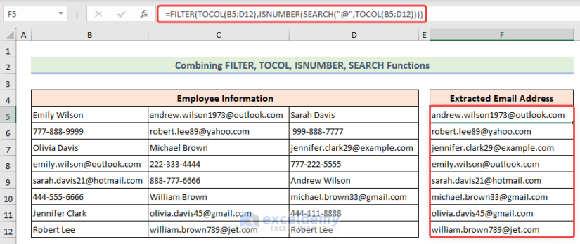
Case 3.2 – Merging FILTER, TOCOL, ISNUMBER, and SEARCH Functions
- Apply the following formula into the result cell:
=FILTER(TOCOL(B5:D12),ISNUMBER(SEARCH("@",TOCOL(B5:D12))))Formula Breakdown
- SEARCH(“@”,TOCOL(B5:D12)
Here the TOCOL function converts the range B5 to D12 into a columnar array. Then the SEARCH function searches for the “@” in each cell on the columnar array.
- ISNUMBER(SEARCH(“@”, TOCOL(B5:D12)))
Here the ISNUMBER function checks if an error occurs in the search operation and returns an array of TRUE or FALSE values.
- FILTER(TOCOL(B5:D12), ISNUMBER(SEARCH(“@”, TOCOL(B5:D12))))
This part applies a filter to the columnar array using the TRUE and FALSE values and returns a new array that includes only the cells where “@” is found.
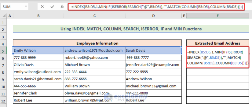
Case 3.3 – Combining INDEX, MATCH, COLUMN, SEARCH, ISERROR, IF, and MIN Functions
- Insert the following formula into a cell and apply it.
=INDEX(B5:D5,1,MIN(IF(ISERROR(SEARCH("@",B5:D5)),"",MATCH(COLUMN(B5:D5),COLUMN(B5:D5)))))
Formula Breakdown
- ISERROR(SEARCH(“@”, B5:D5))
The SEARCH function returns the position of the “@” symbol within each cell, and the ISERROR function checks if an error occurs. If there is an error it returns TRUE, otherwise, it returns FALSE.
- IF(ISERROR(SEARCH(“@”, B5:D5)), “”, MATCH(COLUMN(B5:D5), COLUMN(B5:D5)))
The IF function performs a conditional check. If the result of the previous step is TRUE, it returns an empty string (“”). Otherwise, it proceeds with the MATCH function.
- MATCH(COLUMN(B5:D5), COLUMN(B5:D5))
The MATCH function is used to find the relative position of the current column within the range B5:D5. The COLUMN(B5:D5) part returns an array of column numbers {2, 3, 4}, and MATCH compares each column number with the array itself.
- MIN(IF(ISERROR(SEARCH(“@”, B5:D5)), “”, MATCH(COLUMN(B5:D5), COLUMN(B5:D5))))
Finally, the MIN function is used to find the smallest value from the array returned by the previous step. If there are no errors, it returns the position of the leftmost column with the “@” symbol.
- INDEX(B5:D5,1,MIN(IF(ISERROR(SEARCH(“@”,B5:D5)),””,MATCH(COLUMN(B5:D5),COLUMN(B5:D5)))))
The INDEX function is used to retrieve the value from the range B5:D5. It takes the row number as 1 and the column number as the result of the previous steps.
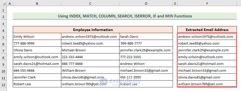
- Drag the Fill Handle down for the rest of the column.
- This extracts the cells with emails from a row.
Read More: Formula to Create Email Address in Excel
Method 4 – Applying VBA Code with a User-Defined Function
- Use Alt + F11 to open the VBA window and insert a module to write a VBA code.
- Inside the module, copy the following code and save it.
Function Extract_Email_Address(emailString As String) As String
emailPattern = "\b[A-Za-z0-9._%+-]+@[A-Za-z0-9.-]+\.[A-Za-z]{2,}\b"
Set regex = CreateObject("VBScript.RegExp")
With regex
.Pattern = emailPattern
.Global = True
End With
Set matches = regex.Execute(emailString)
If matches.Count > 0 Then
Extract_Email_Address = matches(0)
Else
Extract_Email_Address = ""
End If
End Function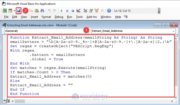
- Go back to the workbook.
- Choose a cell (D5) and copy the formula that uses the newly created user-defined function:
=Extract_Email_Address(B5)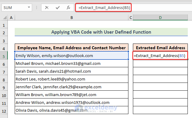
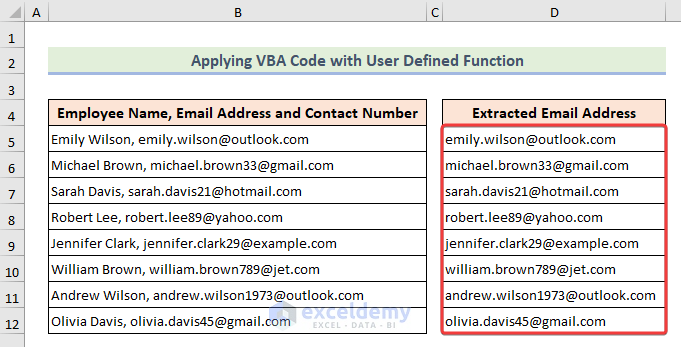
- Hit Enter and drag down the fill handle to extract email addresses.
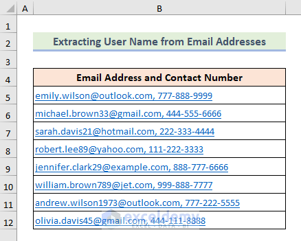
How to Extract Username from Email Addresses in Excel
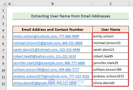
Suppose we have a dataset of Email Addresss and some Contact Numbers with a separator in the same cell. Now, we will extract only the username from the email addresses in Excel.
- Select the whole table and choose the Text to Columns feature from the Data tab.
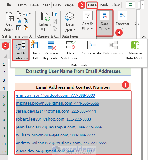
- From the new window, choose Delimited and hit Next.
- Check the Comma option and put @ in the Other section.
- Choose your destination cell, select the columns you don’t need in Data preview, and hit Finish.
- We will get the usernames from the email addresses.
Things to Remember
- On Mac devices, the Flash Fill feature won’t work.
Frequently Asked Questions
1. Can I extract email addresses with specific criteria, such as filtering by domain or filtering out duplicates?
You can filter by domain using text filters or utilize built-in functions to remove duplicates from the extracted email addresses.
2. Can I extract email addresses from multiple Excel files at once?
You can consolidate the data from multiple files into a single Excel file and then extract the email addresses.
3. Can I automate the process of extracting email addresses from Excel?
You can create scripts or programs to extract email addresses from Excel files in a batch process, saving time and effort.
Download Practice Workbook
You can download our practice workbook from here for free!
Related Articles:
- How to Format Addresses in Excel
- How to Organize Addresses in Excel
- Create Email Address with First Initial and Last Name Using Excel Formula

