How to Format Addresses in Excel (4 Easy Methods)

When we copy some addresses from a different file, it is stored in a single cell. As a result, we need to format them in the perfect order for the convenience of other users. We can easily format addresses in several ways using Excel. If you are curious to familiarize yourself with those approaches, download our practice workbook and follow us.

How to Format Addresses in Excel: 4 Easy Methods

To demonstrate the approaches, we consider a dataset of 10 employees of an organization and their residency. The names of the employees’ are in column B, and their addresses are in column C.

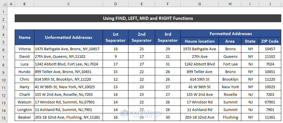
1. Using FIND, LEFT, MID and RIGHT Functions

In this method, we will use the FIND, LEFT, MID, RIGHT, and LEN functions to format addresses in Excel. The procedure is given as follows:

📌 Steps:

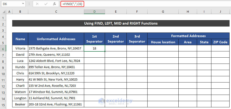
• At the beginning of this process, select cell D6.
• Then, write down the following formula into the cell.

• Press Enter.

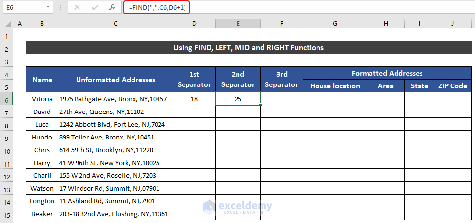
• After that, select cell E6 and write down the following formula in the cell.

• Again, press the Enter.

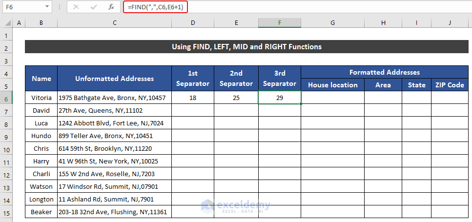
• Similarly, in cell F6, write down the following formula to get the character number of the 3rd separator.

• Press Enter to get its value.

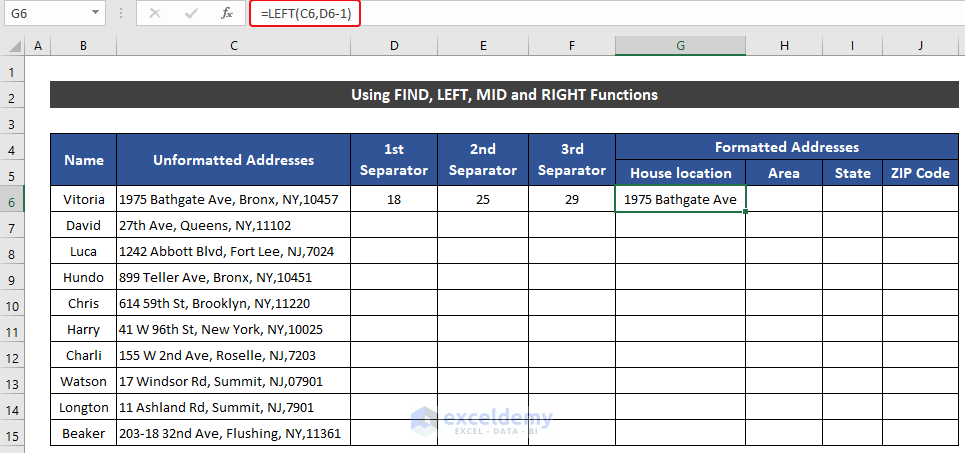
• Now, to get the Home Location, select cell G6 and write down the following formula in the cell. The LEFT function will help us to get the location.

• Then, press Enter to get the Home Location.

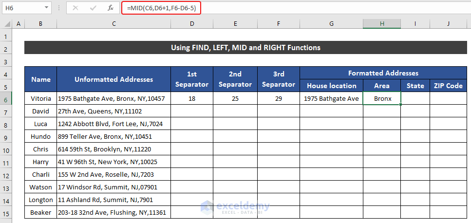
• Next, in cell H6, use the MID function and write down the following formula to get the value of Area.

• Press Enter.

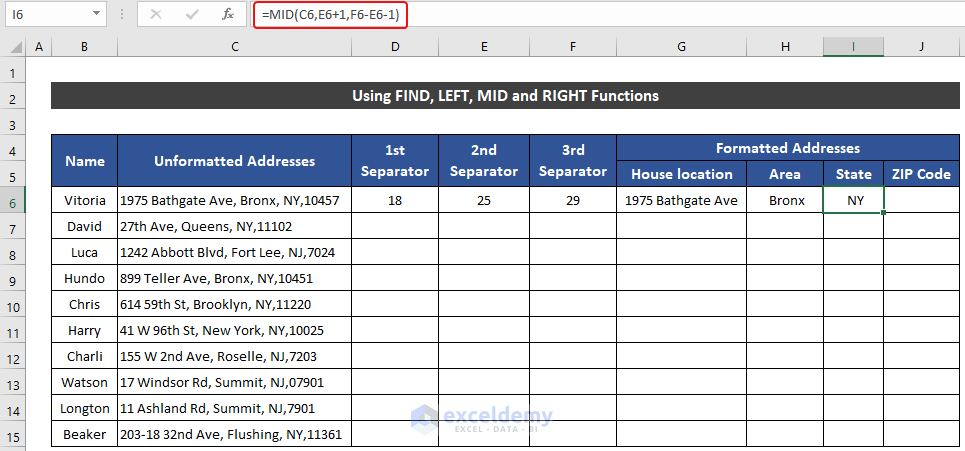
• After that, write down the following formula using the MID function in cell I6 to get the value of the State.

• Press the Enter key to get the value.

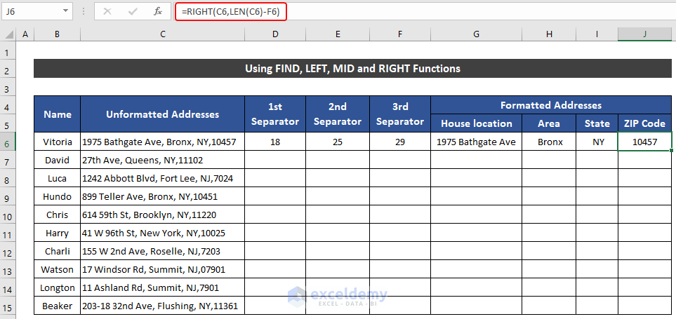
• At last, in cell J6, write down the following formula to get the value of the ZIP Code.

• Similarly, press Enter to get the value.

• Now, select the range of cells D6:J6.
• Double-click on the Fill Handle icon to copy all the formulas up to row 14.

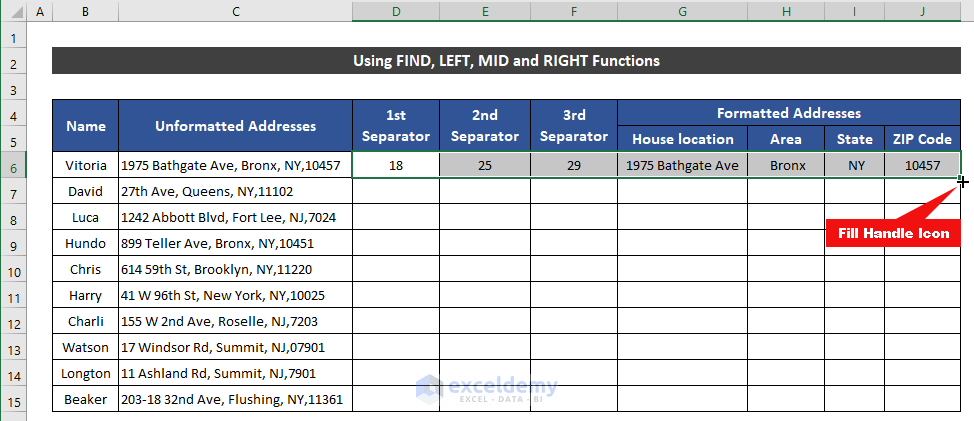
• Finally, you will get all of the unformatted addresses in the correct format.

At last, we can say that all of our formulas worked successfully, and we are able to format addresses in Excel.

Read More: Formula to Create Email Address in Excel

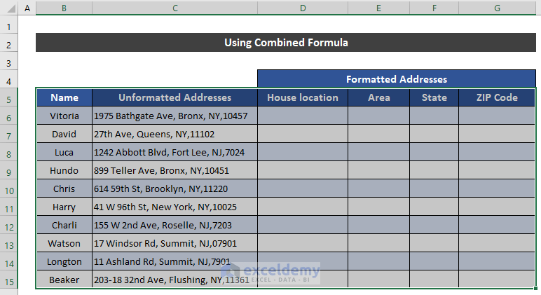
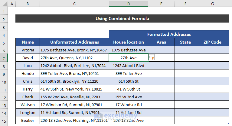
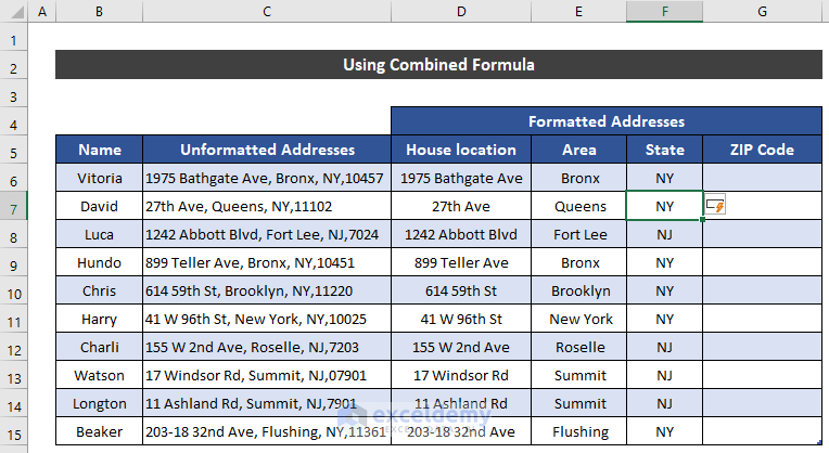
2. Applying Combined Formula to Format Addresses

In this process, we are going to use several combined formulas to format our addresses. The procedure is explained below:

📌 Steps:

• At first, select the range of cells B5:J15.

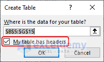
• Then, to convert the data range into a table, press ‘Ctrl+T’.
• As a result, a small dialog box called Create Table will appear.
• Then, check My table has headers option and click OK.

• The table will create and it is going to provide us with some flexibility in the calculation procedure.
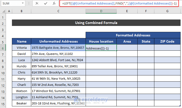
• Now, in cell D6, write down the following formula to get the Home Location. To get the value the LEFT and FIND functions will help us.

• Press Enter and you will see all the cells of the corresponding columns will get the formula. As a result, we don’t need to use the Fill Handle icon anymore.

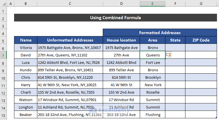
• Then, to get the Area, write down the following formula in cell E6. Here, we will use the MID and FIND functions to get the value.

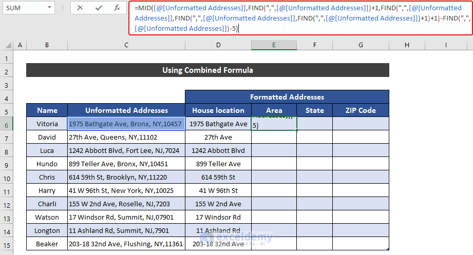
• Again, press Enter.

• After that, in cell F6, write down the following formula for State. For that, we are going to use the MID and FIND functions. Here, our formula will also contain the LEN function.

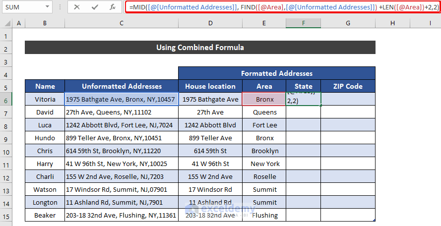
• Similarly, press Enter to get the value.

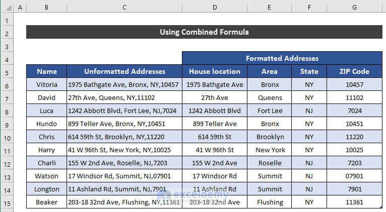
• At last, write down the following formula using the MID and FIND functions in cell G6 to get the ZIP Code.

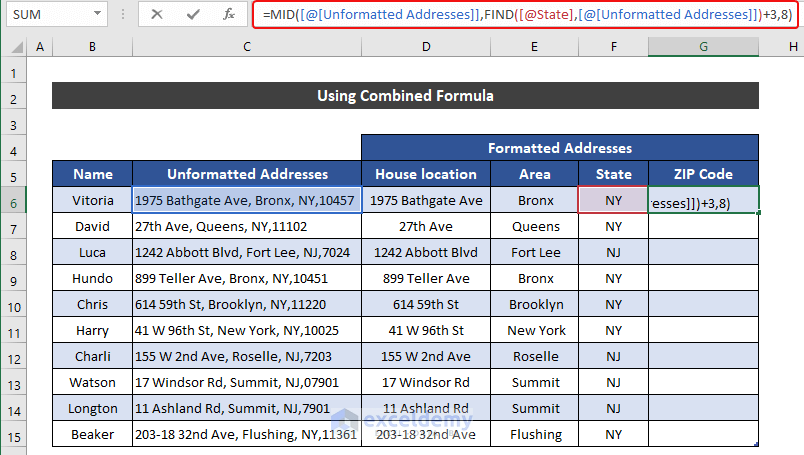
• Press Enter for the last time.

• You will get all the addresses according to our desired format.

In the end, we can say that all of our formulas worked perfectly, and we are able to format addresses in Excel.

Read More: Create Email Address with First Initial and Last Name Using Excel Formula

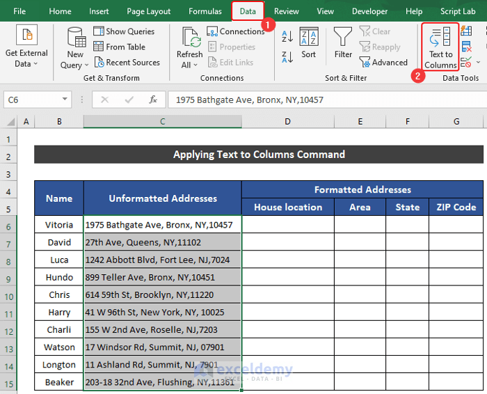
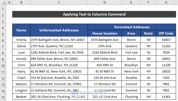
3. Applying Text to Columns Command

In this approach, we will use Excel’s built-in Text to Columns command to format addresses. The steps of this procedure are given below:

📌 Steps:

• First, select the range of cells C5:C14.
• In the Data tab, select the Text to Column command from the Data Tools group.

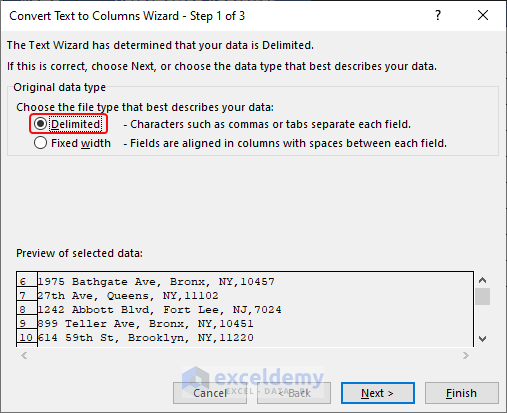
• As a result, the Convert Text to Column Wizard will appear.
• Then, choose the Delimited option and click on Next.

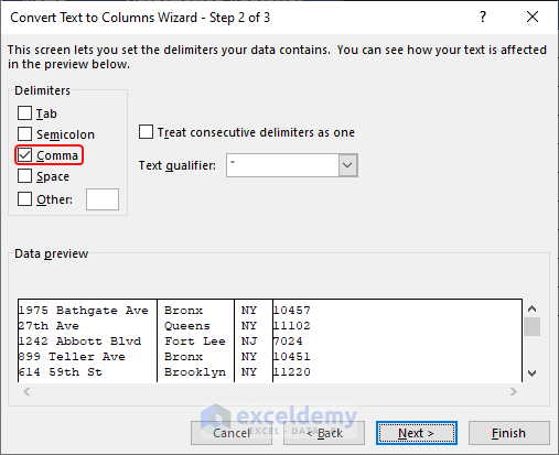
• Next, in the 2nd step, choose Comma as the Delimiters and click Next.

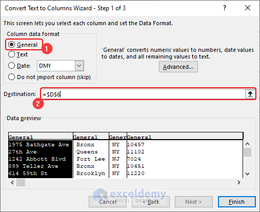
• In the last step, select General in the Column data format section.
• After that, change the Destination cell reference from C6 to D6.
• Finally, click Finish.

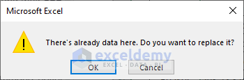
• As we have created a layout for the formatted addresses above row 6, Excel may give you a warning message, like the image shown below. Ignore that and click OK.

• You will get all the entities in your desired format.

Thus, we can say that our method worked successfully, and we are able to format addresses in Excel.

Read More: How to Organize Addresses in Excel

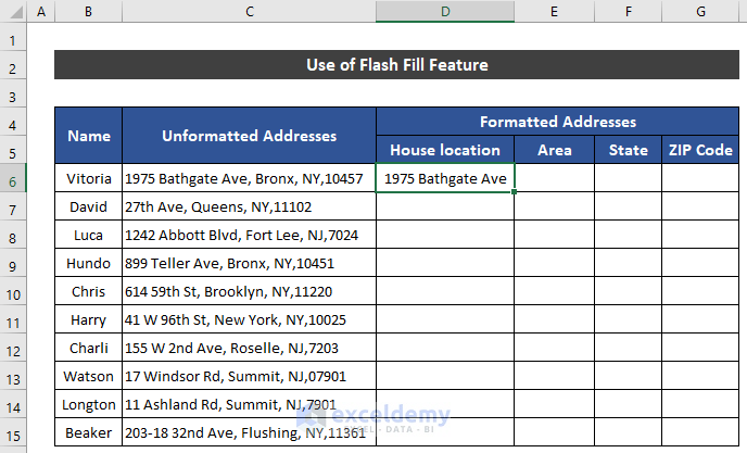
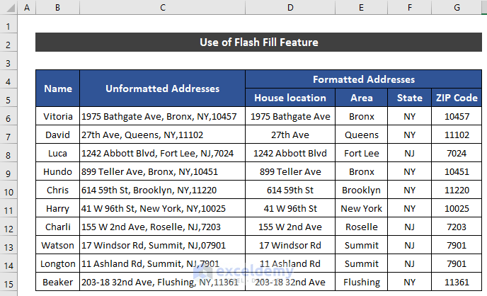
4. Use of Flash Fill Feature

In this method, we will use the Flash Fill feature of Excel to format addresses according to our desire. The steps of this method are given below:

📌 Steps:

• First of all, select cell C6.
• Now, in the Formula Bar, select the text up to the first comma with your mouse.
• Besides it, you can also press the ‘Ctrl+Shift+Right Arrow’ to select the text.
• Press ‘Ctrl+C’ to copy the text.

• Now, select cell D6 and press ‘Ctrl+V’ to paste the text.

• Double-click on the Fill Handle icon to copy the formula up to cell D14.
• After that, click on the drop-down arrow of the Auto Fill Options icon at the bottom of the Fill Handle icon.

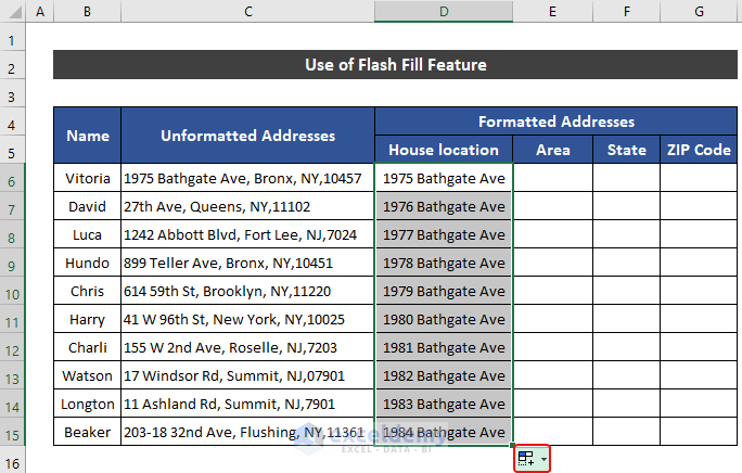
• Then, choose the Flash Fill option.

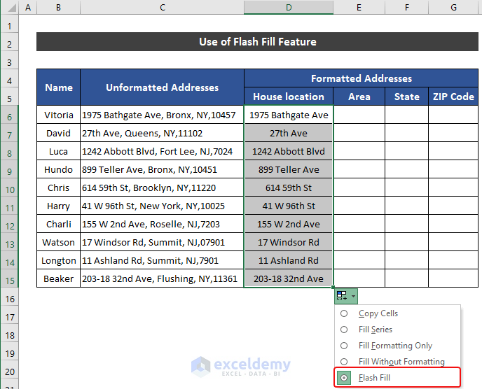
• You will see that every cell up to cell D14 extracted the 1st part of the addresses.
• Similarly, follow the same process for columns titled Area, State, and ZIP Code.
• You will get all the addresses in a proper format.

Finally, we can say that our method worked perfectly, and we can format addresses in Excel.

Read More: How to Make an Address Book in Excel

Download Practice Workbook

Download this practice workbook for practice while you are reading this article.

Conclusion

That’s the end of this article. I hope that this article will be helpful for you and you will be able to format addresses in Excel. Please share any further queries or recommendations with us in the comments section below if you have any further questions or recommendations. Keep learning new methods and keep growing!

Related Articles

• Extracting Email Addresses from Excel
• How to Format a Column for Email Addresses in Excel

<< Go Back to Address Format | Text Formatting | Learn Excel