How to Use SIGN Function in Excel (7 Effective Examples)

Sometimes, we need the sign of any real number. Regarding the demand, Excel provides the SIGN function which returns the sign of number quickly. In this article, I’ll demonstrate the pros and cons of the SIGN function and also its usage.

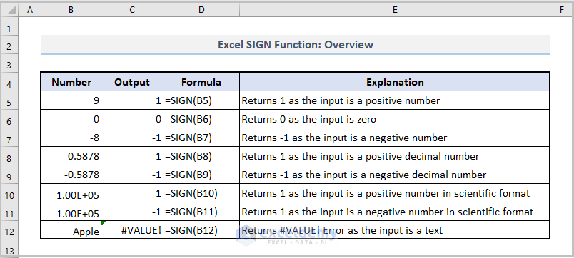
The above figure shows the overview of the utilization of the SIGN function. Now, I’ll show you the uses of the function elaborately.

Download Practice Workbook

Introduction to The SIGN Function

The SIGN is a built-up Excel function, introduced in Excel 2003 version and also available in Excel Microsoft 365, returns the indication of number.

Function Objective

To obtain a number’s sign

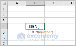
Syntax

SIGN (number)

Arguments Explanation

Return Value

How to Use The SIGN Function in Excel

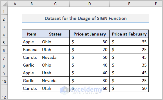
Currently, we have a dataset about the price of some items based on different states of the US. Specifically, the price differs from the two months.

1. Basic Application of The SIGN Function

In the beginning, we’ll see the basic usage of the function that you have already seen in the previous figure. If you input the following formula simply, you’ll get the desired output immediately.

Moreover, you can utilize the SIGN function to change the sign of a list of numbers. For example, if you have a list of numbers like B5:B10, just use the formula below.

Here, the SIGN function returns the sign of the list of numbers into positive.

Read More: 51 Mostly Used Math and Trig Functions in Excel

2. Using The SIGN Function to Compare Two Data

As you see the price of the given items differs, you can compare the two data using the function. Just use the formula below.

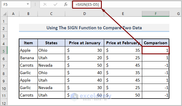
In the case of the first item i.e. Apple, the price is greater in February than that of January. That’s why the output is 1.

Read More: 44 Mathematical Functions in Excel (Download Free PDF)

3. Determining Percentage Change Utilizing Excel SIGN Function

Furthermore, you can get the percentage change using the function. If the second price is higher than the first price, you’ll show a positive percentage number and vice versa.

The formula will be like the following-

Here, E5 is the price of apple in February and D5 is the price of the item in January.

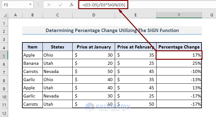
As the price is greater in February than that of January, the function returns 17%.

4. Using SIGN Function Combined with IFERROR Function

The previous method is so easy but has a greater limitation. Because if any input is zero or not available (missing value), the function shows #DIV/0! Error.

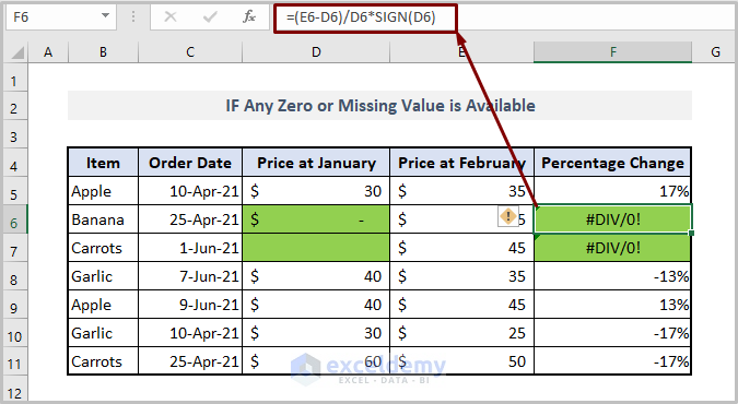
To avoid such a situation, you need to add the IFERROR function first.

So the formula will be

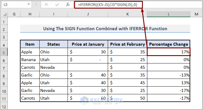
Now, you see that the formula returns 0 instead of the error.

Similar Readings

• How to Use MMULT Function in Excel (6 Examples)
• VBA EXP Function in Excel (5 Examples)
• How to Use TRUNC Function in Excel (4 Examples)
• Use Excel LOG Function (5 Easy Methods)
• How to Use Excel PI Function (7 Examples)

5. Operating Excel SIGN Function Jointly with VLOOKUP

If you want to display the change of the two prices as ‘down’ for negative change, ’equal’ for no change, and ‘up’ for positive change, then you can utilize the VLOOKUP function jointly with the SIGN function.

In that case, the formula will be-

Here, H5 is the price at February, G5 is the price at January, B5:C7 is a table where the sign is fixed to show ‘down’, ‘equal’, and ‘up’, 2 is the column index.

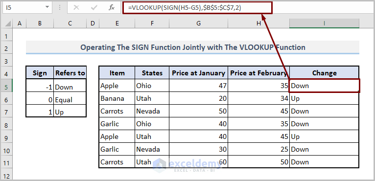
As the second price of ‘Apple’ is lower than the first price, the output shows ‘down’.

6. Employing SIGN Function with SUMPRODUCT Function

Again, if you want the total sales of a specific product of a certain state, you need the combination of SUMPRODUCT and SIGN functions.

Like the following formula.

Here, B5:B15 is the item range, C5:C15 is the range of the states, and D5:D15 is sales for a specific item.

Formula Breakdown:

Firstly, the SIGN((B5:B15=”Apple”)+(C5:C15=”Utah”)) formula sums up if the item “Apple” and state “Utah” are matched, otherwise, it will return 0.

Finally, SUMPRODUCT(–SIGN((B5:B15=”Apple”)+(C5:C15=”Utah”)),D5:D15) returns the total of the desired item and state.

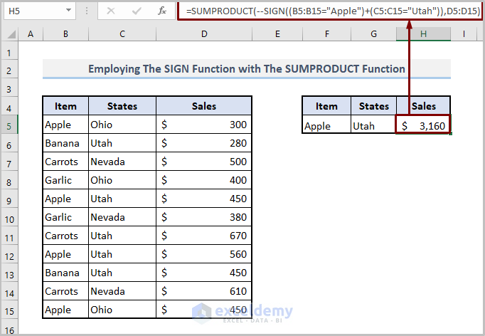
The above picture reveals the total sales of the Apple of Utah state.

Read More: SUMPRODUCT() function in Excel

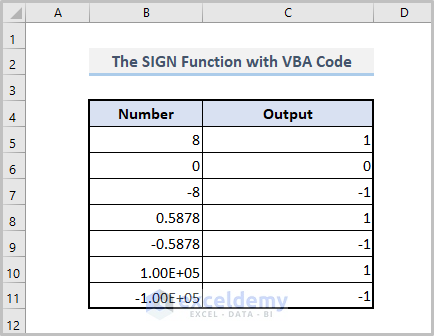
7. Applying The SIGN Function with VBA Code

If you have a larger dataset, it is time-consuming and a little bit boring to get the required result using a formula.

Rather you can utilize the VBA code in Excel which performs the result rapidly and accurately.

Now, let’s see how you can apply the VBA code to get the sign of any real number.

Step 1: 

Firstly, open a module by clicking Developer>Visual Basic>Insert>Module.

Step 2: 

Then, copy the following code in your module.

Sub example_SGN()
Range("C5").Value = Sgn(Range("B5"))
End Sub

Step 3:

Finally, run the code.

Then you’ll see the following output.

Notice:

The following things are essential in the above VBA code.

• Worksheet name: Here, the worksheet name is “SIGN_VBA”
• Logic: The SGN function finds the sign of a number.
• Input Cell: Here, the input cell is B5.
• Output range: The output range is C5.

Things to Remember

Conclusion

This is how you can easily get the sign of any given number. Now, choose the methods based on your requirements. I strongly believe that this article will articulate your journey in Excel. If you have any queries or suggestions, please let me know in The comments section below.

Related Articles

• Use SUBTOTAL Function in Excel (3 Suitable Examples)
• How to Use FACT Function in Excel (2 Suitable Examples)
• Use POWER Function in Excel (5 Suitable Examples)
• How to Use AVERAGEA Function in Excel (10 Examples)
• Use SUMIFS Function in Excel (6 Handy Examples)
• How to Use PRODUCT Function in Excel (With 9 Examples)