How to Refresh Pivot Table in Excel (4 Effective Ways)

In Excel, we use a pivot table to summarize the data rapidly. Pivot tables are the most excellent feature in Excel. But, it does not refresh automatically while modifying or updating data in the worksheet. In this article, we will learn to refresh the pivot table in excel.

Download Practice Workbook

You can download the workbook and practice with them.

Introduction of the Dataset & Pivot Table

The following dataset is about Cars. There are four columns in the dataset. Column B contains the model name of the cars, Column C contains the Brand, Column D contains the color of the car model, and Column E contains the prices of the listed cars. Three bands of cars are listed in the following dataset: Hyundai, Suzuki, and Nissan.

We create a pivot table to summarize the dataset. The pivot table’s Row Labels have the Count of Car Model, Sum of Price, Total Count of Car Model, Total Sum of Price, and its Column Labels have the Colors and the Grand Total. So, now we can easily see the total cars and the total price of all the cars in a compact way.

4 Ways to Refresh Pivot Table in Excel

A pivot table is a trademark in excel which lets the data be reconstructed. But in Excel, the pivot tables could not be updated automatically if we modify the data source.

1. Refresh Pivot with Right Click of the Mouse

Suppose, we don’t want to see the Altima car model which is in the Nissan brand. So, let’s delete row 6. To do this, right-click on the row number and then just click on Delete.

It will delete the row we don’t want to keep on our dataset. Now we can see that the Nissan brand has only one car on the list.

But if we take a look at our created pivot table, the modified data is not updated yet. To refresh the table we just need to follow the steps below.

STEPS:

• Firstly, click anywhere in the pivot table.
• Secondly, right-click on the table and select Refresh.

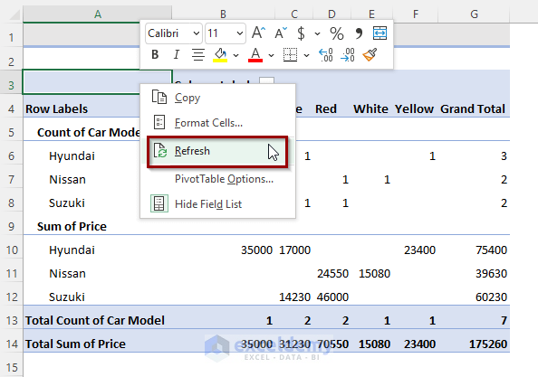
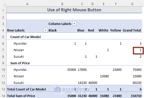
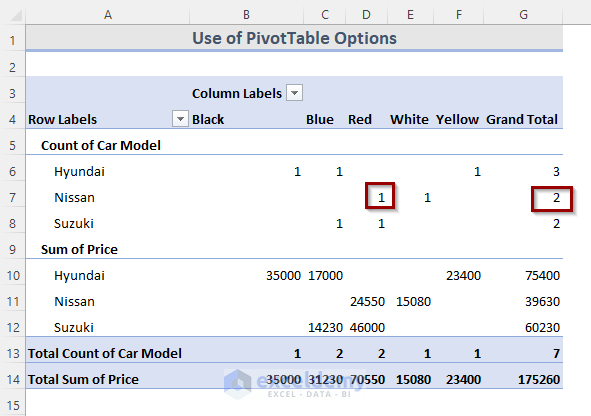
• Finally, this will refresh the pivot table as shown in the picture. As a result, we can see that the Nissan brand now has only one car on the list.

2. Pivot Options to Refresh Automatically While Opening the File

Let’s assume that we want to add the Nissan Altima car again. To do that, right-click on the row where we want to view the inserted data. Then, click on Insert.

This will insert a row, now put the data on the row.

To refresh the updated data to the pivot table, go around with the steps down.

STEPS:

• First, select anywhere in the pivot table.
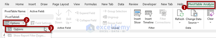
• In the second place, go to the PivotTable Analyze tab from the ribbon.
• After that, from the Options drop-down menu, select Options.

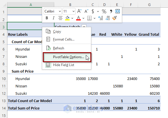
• Instead of doing this, just right-click on the table and select PivotTable Options.

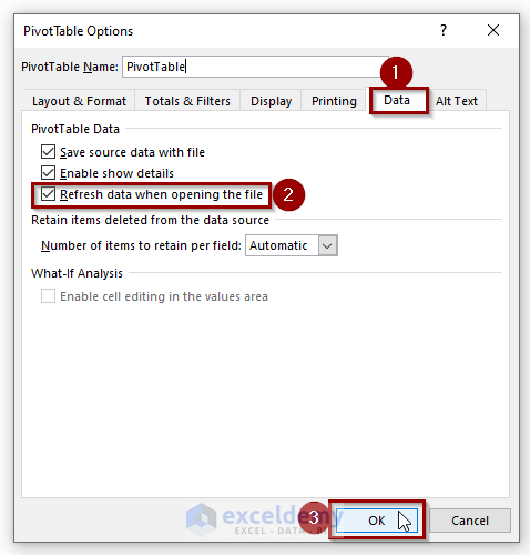
• The PivotTable Options dialog box will appear.
• Consequently, go to the Data menu.
• Next, checkmark the Refresh data when opening the file.
• Then, click on the OK button.

• As a result, now we can view the card which is red now shown in the pivot table. Mainly the pivot table is updated now.

Read More: How to Auto Refresh Pivot Table in Excel

3. Refresh Pivot Data from PivotTable Analyze Tab

To refresh the pivot table as shown in the previous method, we can also use the PivotTable Analyze tab. For this, follow the bellowed steps.

STEPS:

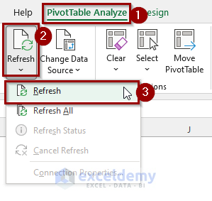
• In the beginning, go to the PivotTable Analyze tab on the ribbon.
• Now, click on the Refresh drop-down menu.
• And, select Refresh.

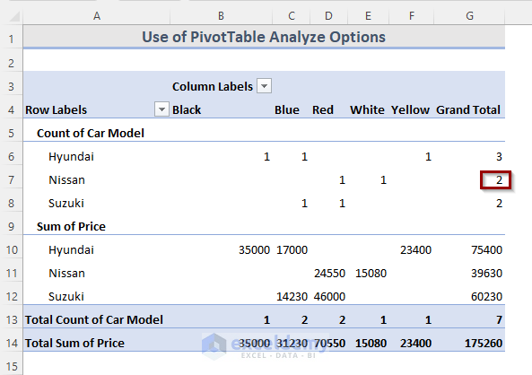
• In the end, we can see the result.

If you have multiple pivot tables in your worksheet, you can refresh all the pivot tables together by clicking on the Refresh All option.

Read More: How to Refresh Chart in Excel (2 Effective Ways)

4. VBA Code to Refresh Pivot table in Excel

We can use a simple VBA code to refresh our pivot table. For this, suppose we delete the Nissan Altima brand again, likewise the earlier methods. To do this, do the same as shown below.

STEPS:

• First, right-click on the sheet where the pivot table is located.
• Second, go to the View Code.

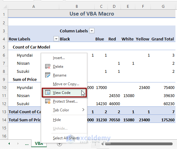
• After that, copy and paste the VBA code below.
• If you have multiple pivot tables in your worksheet.

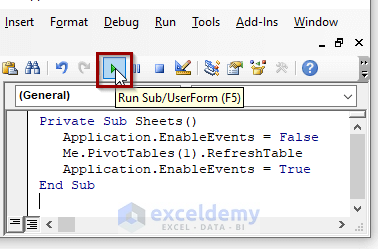
VBA Code:

Private Sub Sheets()
Application.EnableEvents = False
Me.PivotTables(1).RefreshTable
Application.EnableEvents = True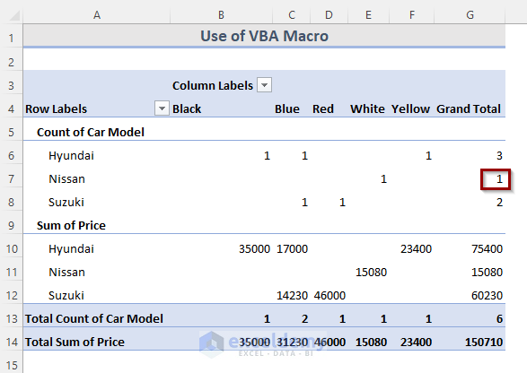
End Sub

• In the end, to Run the code, press the F5 key or click on the Run Sub button.

• This will refresh the pivot table.

Read More: How to Auto Refresh Pivot Table without VBA in Excel (3 Smart Methods)

Things to Remember

• We can easily refresh all the pivot tables with a keyboard shortcut. To do this, just click anywhere on the pivot table then press the Alt + F5 key. It will refresh all the pivot tables on the spreadsheet.

Conclusion

The above methods are guidelines to refresh the pivot tables in Excel. Hope this will help you! If you have any questions, suggestions, or feedback please let us know in the comment section. Or you can have a glance at our other articles in the ExcelDemy.com blog!

Related Articles

• How to Refresh Excel Sheet Automatically (3 Suitable Methods)
• [Fixed!] Excel Cells Not Updating Unless Double Click (5 Solutions)
• How to Disable Background Refresh in Excel (2 Handy Methods)
• Excel VBA: Turn Off Screen Update
• [Solved]: Excel Formulas Not Updating Until Save (6 Possible Solutions)