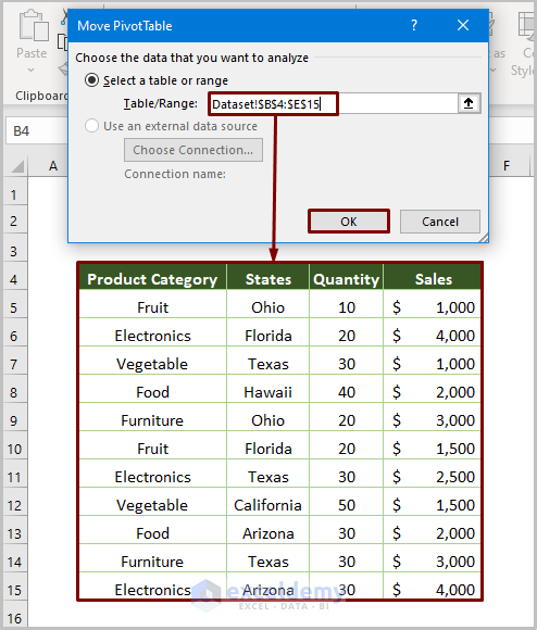
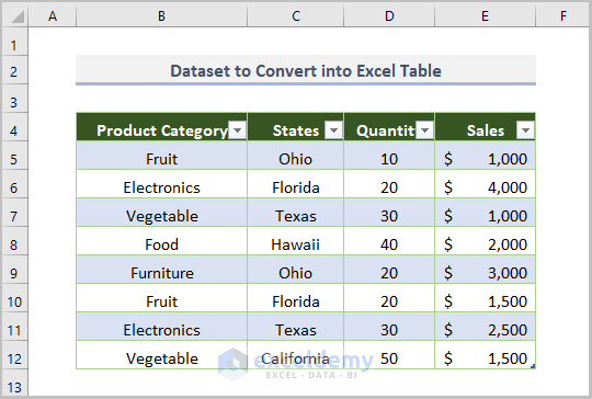
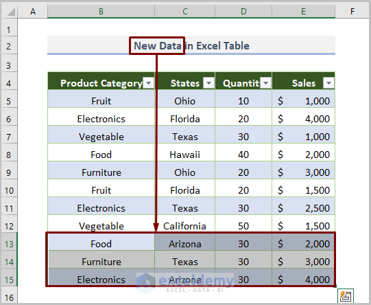
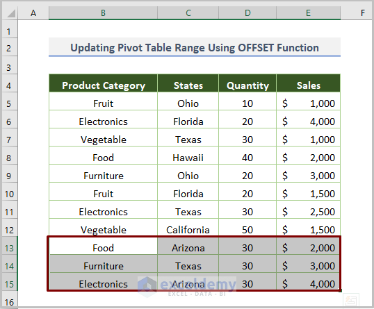
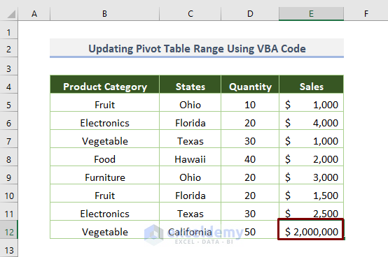
The sample dataset contains the Product Category, Quantity and Sales per State.
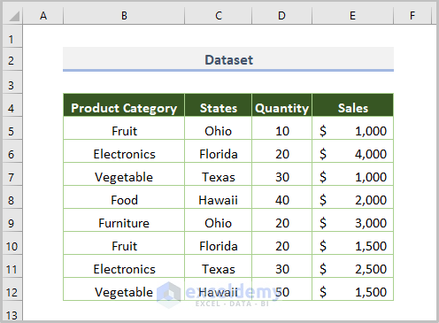
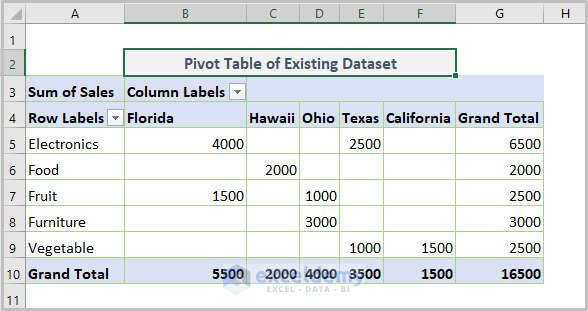
The dataset is configured as a Pivot Table.
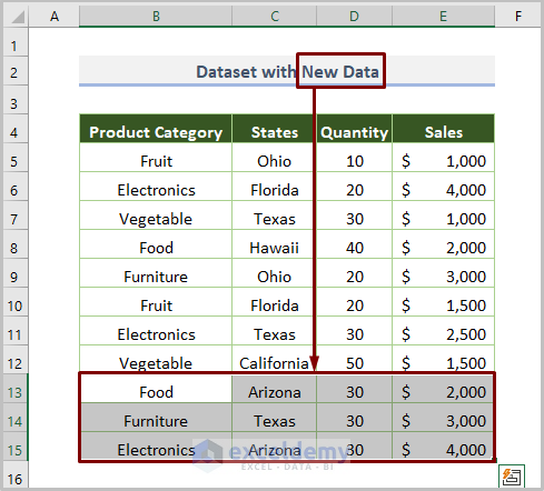
In addition three new rows of data have been added to the dataset which will be updated in the Pivot Table.
Method 1 – Updating the Pivot Table Range Manually by Changing the Data Source
- Select a cell within the Pivot Table.
- Click on the PivotTable Analyze option in the ribbon, then select Change Data Source and then Change Data Source…
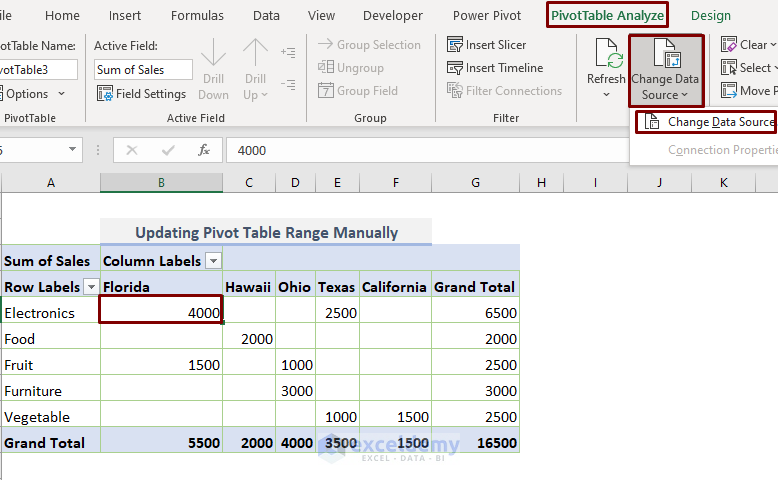
- Move PivotTable option will appear, then change the Table/Range to $B$4:$E$15, and press OK.
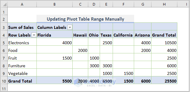
- The Pivot Table will be updated.
Read more: Automatically Update a Pivot Table When Source Data Changes in Excel
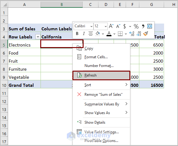
Method 2 – Updating Pivot Table Range by Clicking the Refresh Button
Select a cell within the Pivot Table and then right-click on the mouse or press ALT+F5 then select Refresh from the menu of available options.
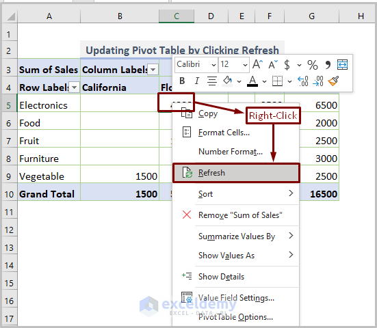
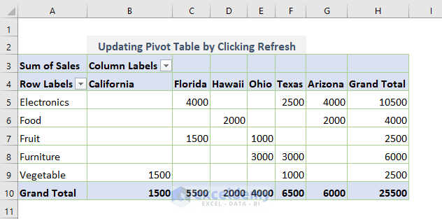
The Pivot Table will update automatically.
Read more: How to Refresh All Pivot Tables in Excel
Method 3 – Updating a Pivot Table Range by Converting to an Excel Table
Steps:
- Select a cell within the dataset and insert a table by clicking the Insert tab > Table.
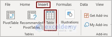
- Alternatively use the CTRL+T keyboard shortcut to create a table.
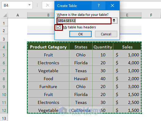
- In the Create Table dialog box enter the Table range (here: $B$4:$E$12) and also check the box My table has headers.
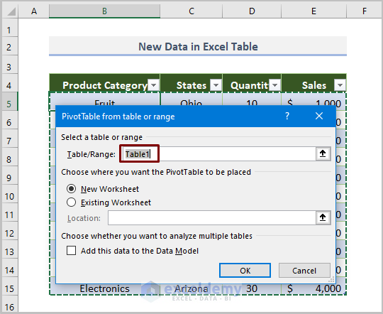
⏩ Now we have to insert a Pivot Table for the above table.
⏩ Make sure the Table/Range is Table1 and press OK.
⏩ Thus, we have created a dynamic Pivot Table range.
⏩ If we input any new data, the above Pivot Table will update automatically including the data.
For example, we want to add the following 3 rows.
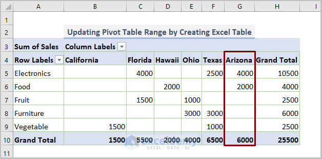
⏩ Then if you select a cell within the Pivot Table, and do right-click on the mouse, and then choose the Refresh option (or press ALT+F5).
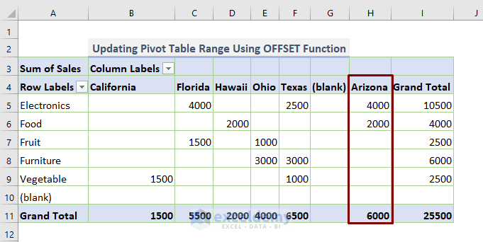
⏩ So, the output will be as follows with the new column Arizona state.
Read more: How to Auto Refresh Pivot Table without VBA in Excel
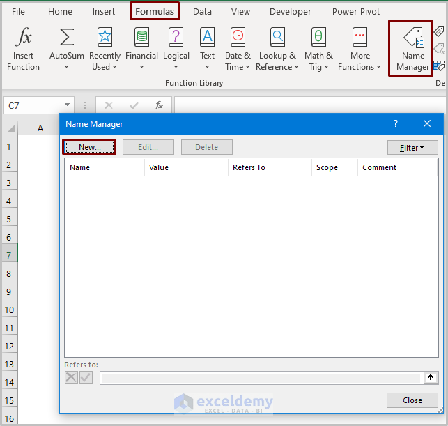
Method 4 – Updating Pivot Table Range Utilizing the OFFSET Function
To create a dynamic range to update the Pivot Table automatically, the Name Manager can be used in combination with OFFSET and COUNTA functions.
Steps:
- Click on the Formulas tab > Name Manager option from the Defined Names ribbon.
- A Name Manager dialog box will appear.
- Click on the New option.
- Set the Name as Source_Data and insert the following formula in the Refers to box
=Dynamic_Range!$B$4:$E$15_Range!$B$4,0,0,COUNTA(Dynamic_Range!$B:$B),COUNTA(Dynamic_Range!$4:$4))Here, the current sheet name is Dynamic_Range, $B$4:$E$15 is the raw data, B4 is the starting cell of the data, $B:$B is column B and $4:$4 is row 4.
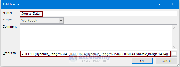
- Click OK.
- In the next dialog box that appears, enter Source_Data in the Table/Range.
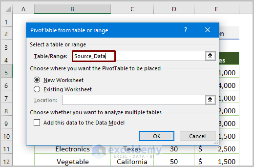
- Click OK to return a new Pivot Table.
Note: If the Table/Range option is not correct, Excel will return a message “the data source is not valid” and no Pivot Table will be created.
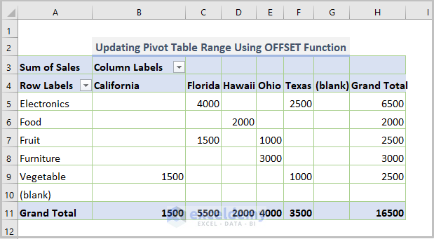
- If we input new data into the raw data table, the Pivot Table will update automatically.
- After adding new data to the dataset press ALT+F5 in the Pivot Table to make it appear here.
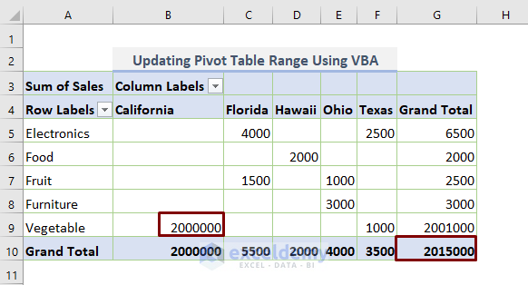
Method 5 – Updating Pivot Table Range Using VBA Code
Step 1:
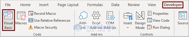
Open a module by clicking Developer > Visual Basic.
Double-click on the Sheet10.
Step 2:
Private Sub Worksheet_Deactivate()
 Sheet9.PivotTables("PivotTable10").PivotCache.Refresh
End Sub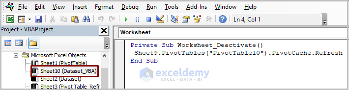
Step 3:
Run the code.
Notes:
- The raw data is saved in Sheet10 (Dataset_VBA).
- The Pivot Table is saved as Sheet9 (PivotTable_VBA).
- Copy the default name of Pivot Table eg PivotTable10.
After changing the sales in the dataset, the Pivot Table now updates automatically.
It is important to note that the Macro cannot retrieve undo history data. To do this the Refresh the data when opening the file option must be turned on.
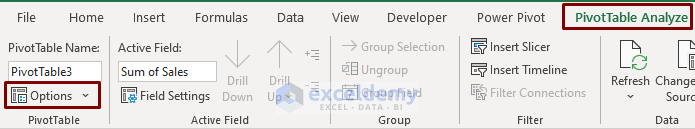
- To do this, click PivotTable Analyze > Options.
- Check the Refresh the data when opening the file option.
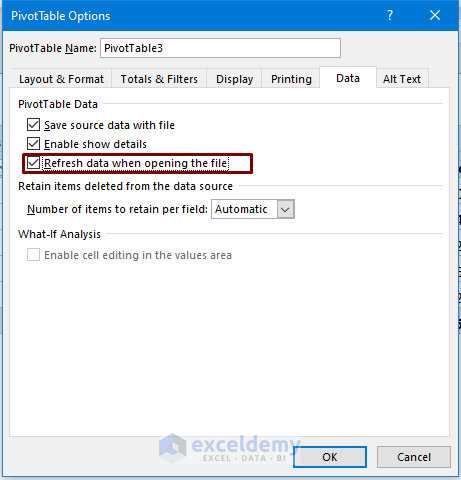
- Click OK.
Download Practice Workbook
Related Articles
- How to Auto Refresh Pivot Table in Excel
- Pivot Table Not Refreshing
- How to Refresh All Pivot Tables with VBA
- How to Refresh Pivot Table with VBA in Excel

