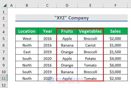
In the table below, there are 5 columns: Location, Year, Fruits, Vegetables, and Sales. For any particular fruits or vegetables, you can use the following methods to match up other values corresponding to this fruit or vegetable from multiple columns.
Method 1 – Using INDEX and MATCH functions on Multiple Columns
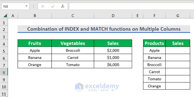
We want the Sales value corresponding to each item in the Products column. To find this value, you have to match it across multiple columns and use an array formula.
Steps:
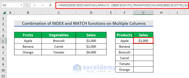
- Select cell G5.
- Enter the following formula:
=INDEX($D$5:$D$7,MATCH(1,MMULT(--($B$5:$C$7=F5),TRANSPOSE(COLUMN($B$5:$C$7)^0)),0))
- Press ENTER to get the output.
Formula Breakdown
- –($B$5:$C$7=F5) → This will generate TRUE/ FALSE for every value in the range depending on the criteria, whether it is met or not and then — will convert TRUE and FALSE into 1 and 0.
- Output: {1,0;0,0;0,0}
- TRANSPOSE(COLUMN($B$5:$C$7)^0) → COLUMN function will create an array with 2 columns and 1 row, and then TRANSPOSE function will convert this array to 1 column and 2 rows. Power zero will convert all of the values in the array to 1
- Output: {1;1}
- MATCH(1,MMULT(–($B$5:$C$7=F5),TRANSPOSE(COLUMN($B$5:$C$7)^0)),0) → The MMULT function will perform matrix multiplication between these two arrays. This result will be used by the MATCH function as the array argument with lookup value 1.
- Output: 1
- INDEX($D$5:$D$7,MATCH(1,MMULT(–($B$5:$C$7=F5),TRANSPOSE(COLUMN($B$5:$C$7)^0)),0)) → Finally, the INDEX function will return the corresponding value.
- Output: 2000
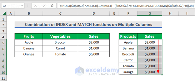
- Drag down the Fill handle to AutoFill the formula.
For other versions except Microsoft 365, you have to press CTRL + SHIFT + ENTER instead of pressing ENTER.
Method 2 – Applying an Array Formula to Match Multiple Criteria
Steps:
- Select cell H7
- Enter the following formula:
=INDEX(F5:F11, MATCH(1, (H4=B5:B11) * (H5=C5:C11) * (H6=D5:D11), 0))
- Press ENTER to get the output.
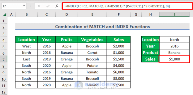
Formula Breakdown
- MATCH(1, (H4=B5:B11) * (H5=C5:C11) * (H6=D5:D11), 0) → Here, 1 is lookup value, H4, H5, H6 are the criterion which will be looked up in B5:B11, C5:C11, and D5:D11 ranges respectively and 0 is for an exact match.
- Output: 2
- INDEX(F5:F11, MATCH(1, (I4=B5:B11) * (I5=C5:C11) * (I6=D5:D11), 0)) → The INDEX function will give the corresponding value.
- Output: 1000
Method 3 – Using a Non-Array Formula to Match Multiple Criteria
Steps:
- Select cell H7.
- Enter the following formula:
=INDEX(F5:F11, MATCH(1, INDEX((H4=B5:B11) * (H5=C5:C11) * (H6=D5:D11), 0, 1), 0))
- Press ENTER to get the output.
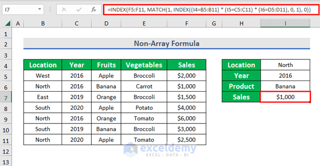
Formula Breakdown
- INDEX((I4=B5:B11) * (I5=C5:C11) * (I6=D5:D11), 0, 1) → This is the lookup_array for the MATCH function.
- Output: {0;1;0;0;0;0;0}
- INDEX(F5:F11, MATCH(1, INDEX((I4=B5:B11) * (I5=C5:C11) * (I6=D5:D11), 0, 1), 0)) → This becomes,
- INDEX(F5:F11, MATCH(1, {0;1;0;0;0;0;0}, 0))
- Output: 1000
Method 4 – Applying an Array Formula to Match Multiple Criteria in Rows and Columns
Steps:
- Select cell H8
- Enter the following formula:
=INDEX(C6:E8, MATCH(H7,B6:B8,0), MATCH(H5&H6,C4:E4&C5:E5,0))
- Press ENTER to get the output.
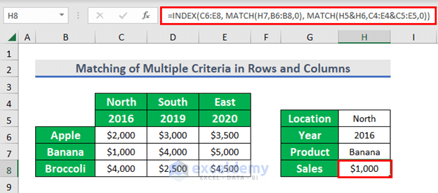
Formula Breakdown
- MATCH(H7, B6:B8,0) → This is used for row-wise matching.
- Output: 2
- MATCH(H5&H6, C4:E4&C5:E5,0) → This is used for column-wise matching.
- Output: 1
- INDEX(C6:E8, MATCH(H7,B6:B8,0), MATCH(H5&H6,C4:E4&C5:E5,0)) → This becomes,
- INDEX(C6:E8, 2, 1,0)
- Output: 1000
Method 5 – Using the VLOOKUP Function
Steps:
- Select the 3 output cells simultaneously: C10, D10, E10
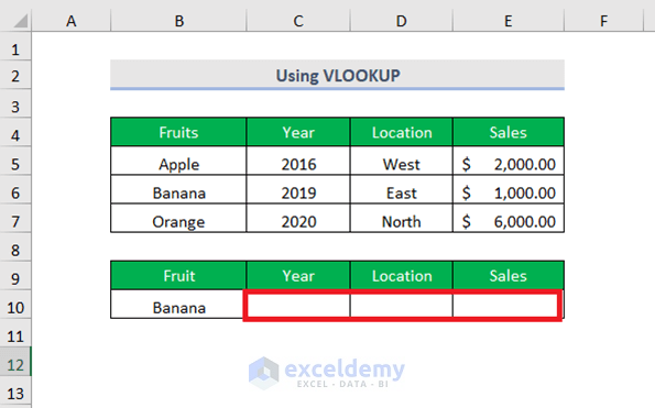
- Enter the following formula:
=VLOOKUP(B10,B4:E7,{2,3,4},FALSE)
- Press ENTER to get the output.
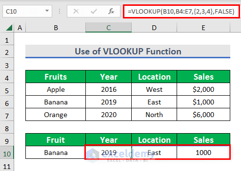
Formula Breakdown
- Here, B10 is lookup_value
- B4:E7 is the table_array, {2,3,4} is the col_index_num
- FALSE is for the Exact match.
Download the Excel Workbook
<< Go Back to Columns | Compare | Learn Excel
Get FREE Advanced Excel Exercises with Solutions!

First method does not work for larger sets of data.
Hi Exceler,
Here, I tried the first method for 50 sets of data and it worked but you have to change the cell references based on your dataset. For your better understanding, I am attaching the images along with the formula.
=INDEX($D$5:$D$30,MATCH(1,MMULT(--($B$5:$C$30=F5),TRANSPOSE(COLUMN($B$5:$C$30)^0)),0))The images of datasets
Here, I used the formula for the entire dataset. I changed the references based on my dataset.
Output for 50 values:
Note: If your dataset is very large kindly send us your dataset
Thanks
Shamima Sultana
Method 1 is very useful!! Thanks!
Dear Excel Nob,
You are most welcome.
Regards
ExcelDemy