Note:
All the operations of this article are accomplished by using the Microsoft Office 365 application.
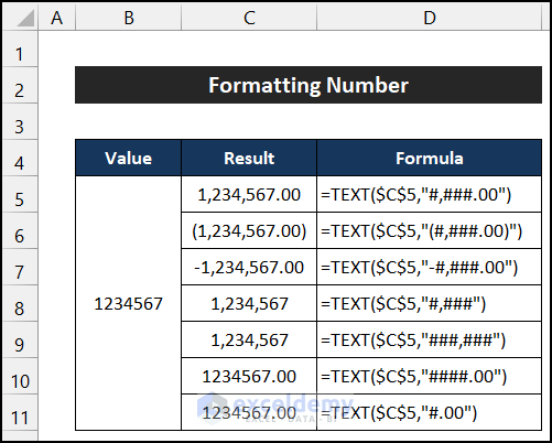
Example 1 – Formatting the Number Value
- Select a cell and copy the formatting formula of your choosing.
To convert the value into the ‘#,###.00’ format, the formula will be:
=TEXT($B$5,"#,###.00")
For converting the value into the ‘(#,###.00)’ format, the formula will be:
=TEXT($B$5,"(#,###.00)")
To convert the value into the ‘-#,###.00’ format, the formula will be:
=TEXT($B$5,"-#,###.00")
For converting the value into the ‘#,###’ format, the formula will be:
=TEXT($B$5,"#,###")
To convert the value into the ‘###,###’ format, the formula will be:
=TEXT($B$5,"###,###")
For converting the value into the ‘####.00’ format, the formula will be:
=TEXT($B$5,"####.00")
To convert the value into the ‘#.00’ format, the formula will be:
=TEXT($B$5,"#.00")
- Press Enter to get the desired cell formatting.
Read More: What Are Excel Function Arguments
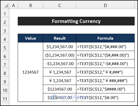
Example 2 – Formatting Currency
- Select any cell and enter the formula you need.
To convert the value into the ‘$#,###.00’ format, the formula will be:
=TEXT($B$5,"$#,###.00")
For converting the value into the ‘($#,###.00)’ format, the formula will be:
=TEXT($B$5,"($#,###.00)")
To convert the value into the ‘-$#,###.00’ format, the formula will be:
=TEXT($B$5,"-$#,###.00")
For converting the value into the ‘¥#,###’ format, the formula will be:
=TEXT($B$5,"¥#,###")
To convert the value into the ‘¥###,###’ format, the formula will be:
=TEXT($B$5,"¥###,###")
For converting the value into the ‘$####.00’ format, the formula will be:
=TEXT($B$5,"$####.00")
To convert the value into the ‘$#.00’ format, the formula will be:
=TEXT($B$5,"$#.00")
- Press Enter to get the desired currency formatting.
Read More: Top Excel Functions and Features for Management Consultants
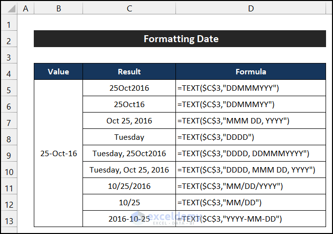
Example 3 – Formatting Date
- Select any cell and copy the necessary formula.
To convert the date into the ‘DDMMMYYY’ format, the formula will be:
=TEXT($B$5,"DDMMMYYY")
For converting the date into the ‘DDMMMYY’ format, the formula will be:
=TEXT($B$5,"DDMMMYY")
To convert the date into the ‘MMM DD, YYYY’ format, the formula will be:
=TEXT($B$5,"MMM DD, YYYY")
For converting the date into the ‘DDDD’ format, the formula will be:
=TEXT($B$5,"DDDD")
To convert the date into the ‘DDDD,DDMMMYYYY’ format, the formula will be:
=TEXT($B$5,"DDDD, DDMMMYYYY")
For converting the date into the ‘DDDD, MMM DD, YYYY’ format, the formula will be:
=TEXT($B$5,"DDDD, MMM DD, YYYY")
To convert the date into the ‘MM/DD/YYYY’ format, the formula will be:
=TEXT($B$5,"MM/DD/YYYY")
For converting the date into the ‘MM/DD’ format, the formula will be:
=TEXT($B$5,"MM/DD")
To convert the date into the ‘YYYY-MM-DD’ format, the formula will be:
=TEXT($B$5,"YYYY-MM-DD")
- Press Enter to get the desired date formatting.
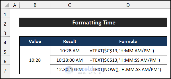
Example 4 – Formatting Time
- Select any cell and enter one of the following formulas based on your needs.
To convert the time into the ‘H:MM AM/PM’ format, the formula will be:
=TEXT($B$5,"H:MM AM/PM")
For converting the time into the ‘H:MM:SS AM/PM’ format, the formula will be:
=TEXT($B$5,"H:MM:SS AM/PM")
To convert the time into the ‘H:MM:SS AM/PM’ format, the formula will be:
=TEXT(NOW(),"H:MM:SS AM/PM")
We will also use the NOW function.
- Press Enter to get the desired time formatting.
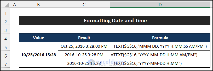
Example 5 – Formatting Combined Date and Time
- Select any cell and enter any of the formulas below, according to your needs.
To convert the both date and time into the ‘MMM DD, YYYY H:MM:SS AM/PM’ format, the formula will be:
=TEXT($B$5,"MMM DD, YYYY H:MM:SS AM/PM")
For converting both date and time into the ‘YYYY-MM-DD H:MM AM/PM’ format, the formula will be:
=TEXT($B$5,"YYYY-MM-DD H:MM AM/PM")
To convert both date and time into the ‘YYYY-MM-DD H:MM’ format, the formula will be:
=TEXT($B$5,"YYYY-MM-DD H:MM")
- Press Enter to format the value.
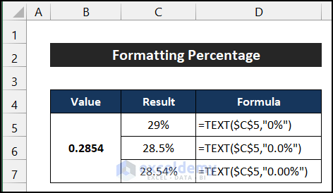
Example 6 – Formatting Percentage
- Select any cell and enter one of the following formulas.
To convert the value into the ‘0%’ format, the formula will be:
=TEXT($B$5,"0%")
For converting the value into the ‘0.0%’ format, the formula will be:
=TEXT($B$5,"0.0%")
To convert the value into the ‘0.00%’ format, the formula will be:
=TEXT($B$5,"0.00%")
- Press Enter to get the desired percentage formatting.
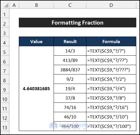
Example 7 – Formatting a Fraction Number
- Select any cell and enter any of the formulas below.
To convert the value into the ‘?/?’ fraction format, the formula will be:
=TEXT($B$5,"?/?")
For converting the value into the ‘?/??’ fraction format, the formula will be:
=TEXT($B$5,"?/??")
To convert the value into the ‘?/???’ fraction format, the formula will be:
=TEXT($B$5,"?/???")
For converting the value into the ‘?/2’ fraction format, the formula will be:
=TEXT($B$5,"?/2")
To convert the value into the ‘?/4’ fraction format, the formula will be:
=TEXT($B$5,"?/4")
For converting the value into the ‘?/8’ fraction format, the formula will be:
=TEXT($B$5,"?/8")
To convert the value into the ‘?/16’ fraction format, the formula will be:
=TEXT($B$5,"?/16")
For converting the value into the ‘?/10’ fraction format, the formula will be:
=TEXT($B$5,"?/10")
To convert the value into the ‘?/100’ fraction format, the formula will be:
=TEXT($B$5,"?/100")
- Press Enter to get the desired percentage formatting.
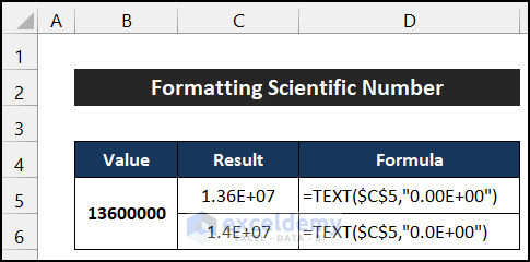
Example 8 – Formatting a Scientific Number
- Select a cell and enter any of the formulas below.
To convert the value into the ‘0.00E+00’ format, the formula will be:
=TEXT($B$5,"0.00E+00")
For converting the value into the ‘0.0E+00’ format, the formula will be:
=TEXT($B$5,"0.0E+00")
- Press Enter to get the formatted value.
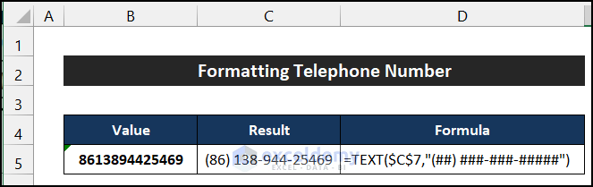
Example 9 – Formatting a Telephone Number
- Select a cell and copy the formula below.
To convert the value into the ‘(##) ###-###-#####’ format, the formula will be:
=TEXT($B$5,"(##) ###-###-#####")
- Press Enter to format your value as a telephone number.
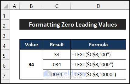
Example 10 – Formatting a Number With a Leading Zero
- Select any cell and write down one of the following formulas:
To convert the value into the ‘00’ format, the formula will be:
=TEXT($B$5,"00")
For converting the value into the ‘000’ format, the formula will be:
=TEXT($B$5,"000")
To convert the value into the ‘0000’ format, the formula will be:
=TEXT($B$5,"0000")
- Press Enter to get the desired percentage formatting.
Overview of VBA Format Function
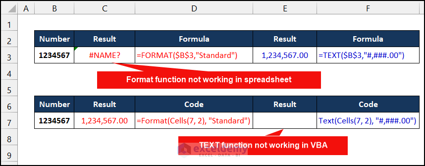
Format is a VBA function. You cannot find or use it in an Excel spreadsheet.
⏺ Function Objective:
This function is generally used to change the format of a cell value through the VBA.
⏺ Syntax:
Format(Expression, [Format])
⏺ Arguments Explanation:
| Argument | Required/Optional | Explanation |
|---|---|---|
| Expression | Required | Expression is the text string or cell value you want to format. |
| Format | Optional | This is the desired cell formatting. |
⏺ Return:
After running the code, the function will show the cell value with the desired formatting.
⏺ Availablity:
Excel for Office 365, Excel 2019, Excel 2016, Excel 2013, Excel 2011 for Mac, Excel 2010, Excel 2007, Excel 2003, Excel XP, Excel 2000.
VBA Format Function to Format a Cell Value: 5 Suitable Examples
Here, we will demonstrate 5 easy examples for showing the format changing of cell values through the VBA Format Function. The examples are shown below step-by-step:
Example 1 – Formatting a Number
Steps:
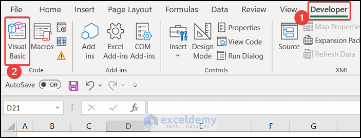
- Go to the Developer tab and click on the Visual Basic button. If you can’t find this tab, you must enable it first. Alternatively, you can press ‘Alt+F11’ to open the Visual Basic Editor.
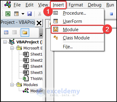
- Click on the Insert tab in the pop-up window and select the Module option.
- Copy the following visual code to the empty editor box:
Sub Format_Number()
Worksheets(11).Activate
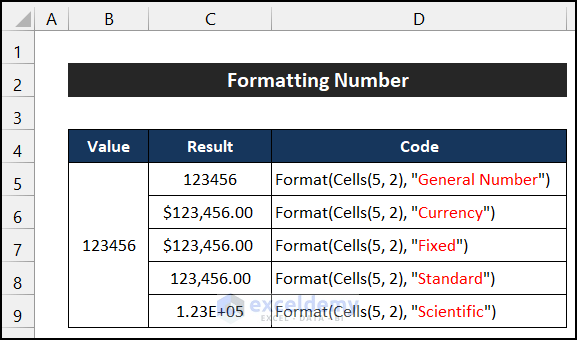
Cells(5, 2) = 123456
Cells(5, 3) = Format(Cells(5, 2), "General Number")
Cells(6, 3) = Format(Cells(5, 2), "Currency")
Cells(7, 3) = Format(Cells(5, 2), "Fixed")
Cells(8, 3) = Format(Cells(5, 2), "Standard")
Cells(9, 3) = Format(Cells(5, 2), "Scientific")
End Sub- Press ‘Ctrl+S’ to save the code.
- Close the Editor tab.
- Navigate to the the Developer tab and click on the Macros button in the Code section.
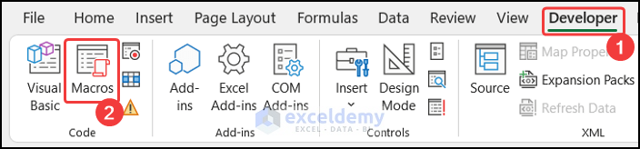
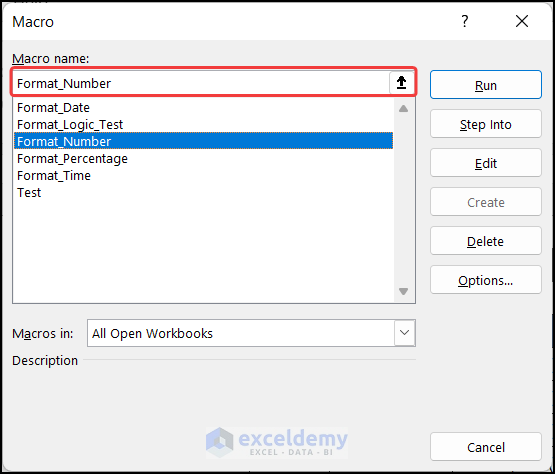
- Select the Format_Number option in the Macro dialog box.
- Click the Run button to run the code.
- The number will now be displayed in different formats.
Example 2 – Formatting Percentage
Steps:
- Go to the Developer tab and click on the Visual Basic button. If you can’t see the tab, you must enable it first. You can also press ‘Alt+F11’ to launch the Visual Basic Editor.
- Head to the Insert tab in the pop-up dialog box and select the Module option.
- Enter the following visual code into the empty editor box:
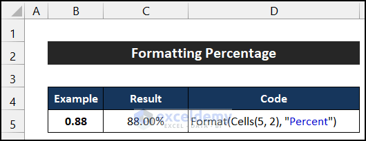
Sub Format_Percentage()
Worksheets(12).Activate
    Cells(5, 2) = 0.88
    Cells(5, 3) = Format(Cells(5, 2), "Percent")
End Sub- Press ‘Ctrl+S’ to save the code.
- Close the Editor tab.
- Go to the Developer tab and click on the Macros button in the Code section.
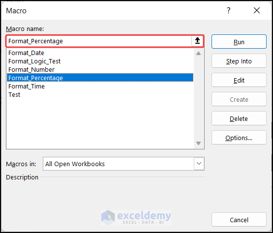
- Select the Format_Percentage option in the dialog box titled Macro
- Click the Run button to run the code.
- The number will now be shown in the percentage format.
Example 3 – Formatting for a Logic Test
Steps:
- Go to the Developer tab and click on the Visual Basic button. If you don’t have the Developer tab, enable it first. You can also press ‘Alt+F11’ to open the Visual Basic Editor.
- In the pop-up dialog box, navigate to the Insert tab and choose the Module option.
- Copy the following visual code to the empty editor box:
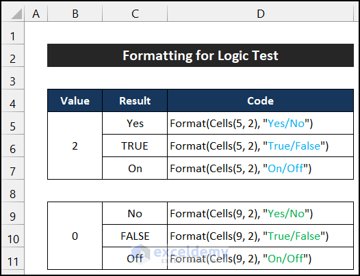
Sub Format_Logic_Test()
Worksheets(13).Activate
  Cells(5, 2) = 2
  Cells(5, 3) = Format(Cells(5, 2), "Yes/No")
  Cells(6, 3) = Format(Cells(5, 2), "True/False")
  Cells(7, 3) = Format(Cells(5, 2), "On/Off")

  Cells(9, 2) = 0
  Cells(9, 3) = Format(Cells(9, 2), "Yes/No")
  Cells(10, 3) = Format(Cells(9, 2), "True/False")
  Cells(11, 3) = Format(Cells(9, 2), "On/Off")
End Sub- Press ‘Ctrl+S’ to save the code.
- Close the Editor tab.
- Go to the Developer tab and click on Macros from the Code group.
- Select the Format_Logic_Test option from the Macro pop-up window and click on the Run button.
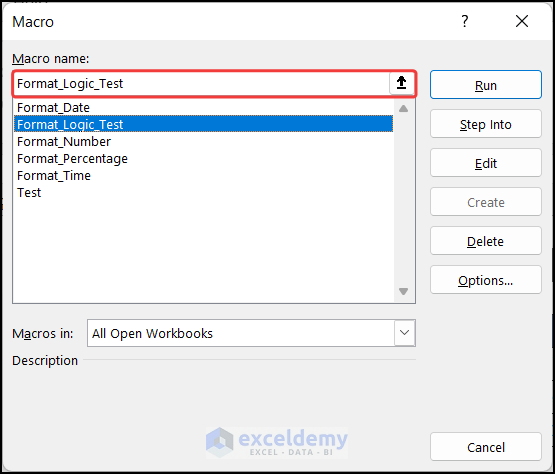
- You should see the result below.
Example 4 – Formatting Date
Steps:
- Go to the Developer tab and click on the Visual Basic button. If you don’t have this tab, you must enable it first. Alternatively, you can press ‘Alt+F11’ to open the Visual Basic Editor.
- Navigate to the Insert tab in the pop-up window and select the Module option.
- Enter the following visual code into the empty editor box:
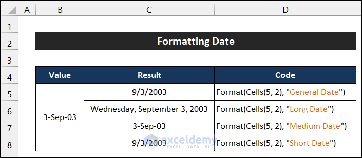
Sub Format_Date()
Worksheets(14).Activate
  Cells(5, 2) = "Sep 3, 2003"
  Cells(5, 3) = Format(Cells(5, 2), "General Date")
  Cells(6, 3) = Format(Cells(5, 2), "Long Date")
  Cells(7, 3) = Format(Cells(5, 2), "Medium Date")
  Cells(8, 3) = Format(Cells(5, 2), "Short Date")
End Sub- Press ‘Ctrl+S’ to save the code.
- Close the Editor tab.
- Go to the Developer tab and click on Macros from the Code group.
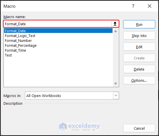
- Select the Format_Date option under Macro name.
- Click on Run.
- You will see dates in multiple formats.
Example 5 – Formatting Time Value
Steps:
- Go to the Developer tab and click on the Visual Basic button. If you don’t have the Developer tab, enable it first. You can also press ‘Alt+F11’ to open the Visual Basic Editor.
- Go to the Insert tab in the pop-up dialog box and click on the Module option.
- Copy the following visual code to the empty editor box:
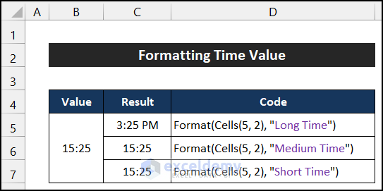
Sub Format_Time()
Worksheets(15).Activate
  Cells(5, 2) = "15:25"
  Cells(5, 3) = Format(Cells(5, 2), "Long Time")
  Cells(6, 3) = Format(Cells(5, 2), "Medium Time")
  Cells(7, 3) = Format(Cells(5, 2), "Short Time")
End Sub- Press ‘Ctrl+S’ to save the code.
- Close the Editor tab.
- Head back to the Developer tab and click on Macros in the Code section.
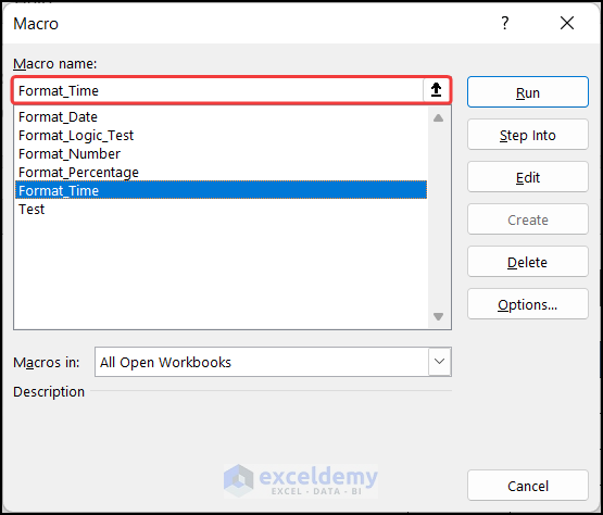
- Select the Format_Time option and click on the Run button.
- You will see the time value in different formats.
Things You Should Know
- The TEXT function will be applicable only in the Excel spreadsheet. You cannot use this function in the VBA environment. If you try to use the function in your VBA workspace, Excel will show you an error, and the code will not run.
- You can use the Format function only in the VBA workspace. Inside the Excel worksheet, you won’t be able to find any function called Format.
Download Practice Workbook
Download this workbook to practice while reading this article.
Related Articles
- Compatibility Function in Excel
- Most Useful and Advanced Excel Functions List
- 51 Mostly Used Math and Trig Functions in Excel
<< Go Back to Excel Functions | Learn Excel
Get FREE Advanced Excel Exercises with Solutions!

Good day. Is it right that once I put a number or date in a Text format, I am unable to calculate with it ?
Yes, when a number or date is placed in a cell in Text format, you cannot calculate with them.
Thanks. I have another question.
Let’s say I have a problem within an existing sheet or workbook and try to ask you for a solution by texting you (f.e. in this comment space). This might be unconvincing for you, because, either I don’t know how to formulate my problem or you can’t see the building of my sheet/formulas etc.
Is there a way to send you example files, where you can go through and see where I made a ridiculous mistake and you have the power to help me with your immense knowledge ?
Thank you ROGER for reaching out to us. Sure you can send me your files at my mail: [email protected]
I’ll be happy to help you.
WHOW. I see you reacted to my former post for the possibility to download your posts as PDF for later evaluation.
Great job.
Thanks a lot for this unique opportunity.
I like your posts very much, compared to other, similar newsletters, this is the easiest to handle.
Congrats from here…
Thank you Roger for the beautiful comment.
Nice! You solved my question in seconds after googling a question about how to format a cell value. Thank you for the clear examples!
Welcome WILLIAM, it’s always a pleasure to hear that we were of any help to you.
Thanks for the nice comment. Good luck.
Yup, me, too! You gave me the concise use for TEXT. Thank you.
Thanks, Mike for your nice comment.