How to Compare Sheets Side by Side in Excel (5 Examples)

In this article, we will show you how to use Excel to compare sheets side by side. Comparing various datasets at the same time is a very common scenario in our lives. We need to compare sheets side by side to get a clear idea of a topic. The method of comparing sheets side by side varies and entirely depends on the user. The user might want to view the sheets side by side to compare them with their own eyes. Or they can implement various formulas to spot different areas instantly.

Moreover, they have a VBA macro to compare the side of the sheet by side in Excel by highlighting the other values. Below, we showed how, in Microsoft Excel, users can compare the sides of the worksheet side by side by following various methods.

Below, we showed methods where we compared the sheet side by side and highlighted the cell values that were different from each other.

Compare Sheets Side by Side in Excel: 5 Useful Examples

Here we are giving five separate examples to compare sheets side by side. To avoid any kind of compatibility issue, users are advised to use the Microsoft 365 edition.

1. Using View Tab to Compare Sheets Side by Side in Excel

The most common and most accessible way a person can view the worksheets is by using the View Side by Side option from the View tab.

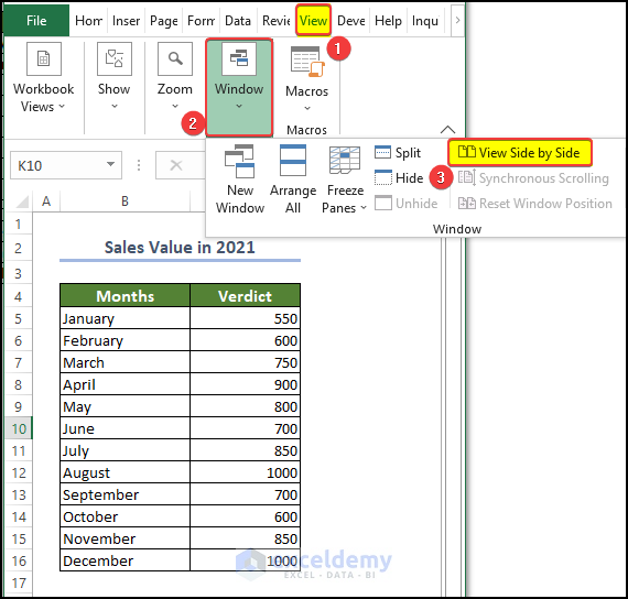
First, go to the View tab> Window > View Side by Side command.

Then, in the Compare Side by Side dialog box, select the other worksheet in another open workbook.
Press OK after this.

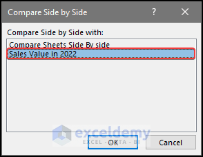
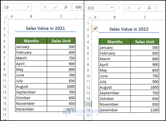
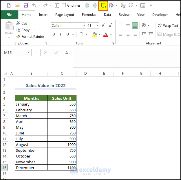
After selecting the Sales Value in 2022, we can see that both of the worksheets are now open simultaneously and scroll synchronously.

Note: Both of the worksheets need to be open at the same time before clicking on the Side by Side.

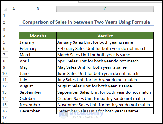
2. Using Formula to Find Differences in Values and Compare Sheets Side by Side in Excel

We can use formulas that consist of the IF function to compare values side by side in Excel.

For this, we need to enter the following formula into the C5 cell. In the video shown below.

=IF('[Sales Value in 2021.xlsm]2021 Sales Value'!C5='[Sales Value in 2022.xlsm]2022 Sales Value'!C5, B5& " Sales Unit for both year is same", B5& " Sales Unit for both years do not match")

After pressing the Enter button, we can see that the comparison made between the worksheet and the verdict made based on them is presented in cell C5.
Then drag the fill handle to cell C16.
After dragging cell C16, we will see that the range of cells C5:C16 will be filled in with the verdict based on the worksheet values.

3. Use of Compare and Merge Workbooks Command to Compare Sheets Side by Side in Excel

In this method, we can use the compare and merge method to compare multiple workbooks and then merge them.

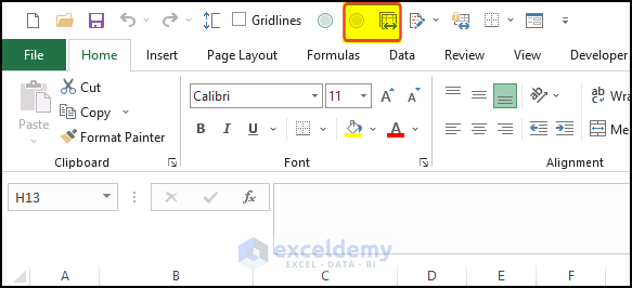
But first, you need to add the Compare and Merge tool to the Quick Access Toolbar.
First, click on the Options button. Then in the Options window, click on the quick access toolbar.
Then select All Commands from the Choose Commands form.
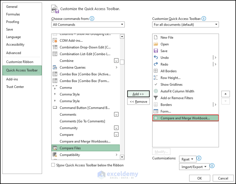
Then select Compare and Merge Workbooks (Legacy) and then click on the Add button.

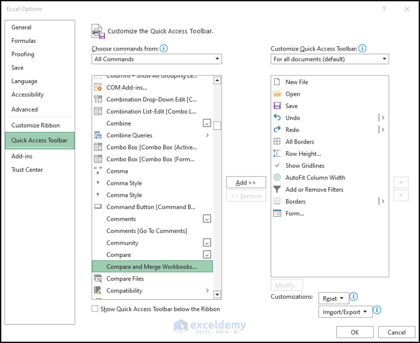
After clicking the Add button, we can see that the tool is on the right side of the window.
Press OK after this.

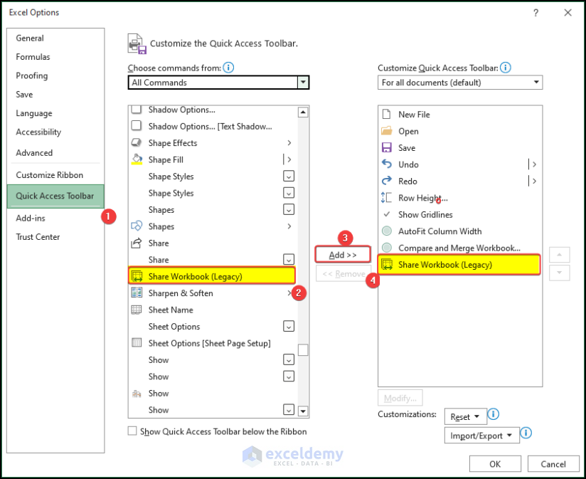
After that, we need to add another tool named Shared Workbook(Legacy) in the quick access toolbar.
Select that tool Shared Workbook(Legacy) and then press Add to add the command on the right side of the workbook.
Click OK after this.

We can see the added tools in the Quick Access Toolbar.

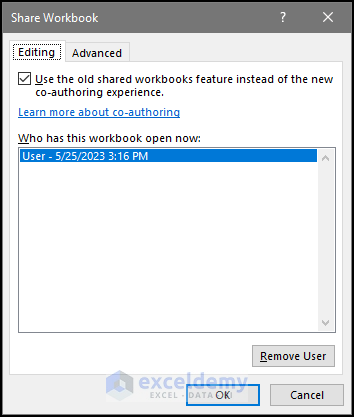
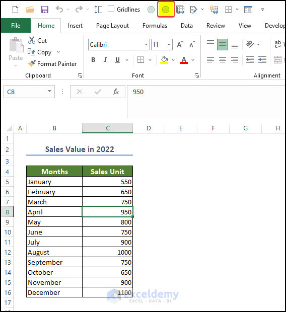
Then, click on the Share Workbook(Legacy) command.

After clicking on the Share Workbook tool on the Quick Access Toolbar, users can see that there is a window in which they have to select the user of the computer right now.
Click OK after this.

Repeat the same process for the second file also.
Then, in the Quick Access Toolbar, click on the Compare and Merge tool.

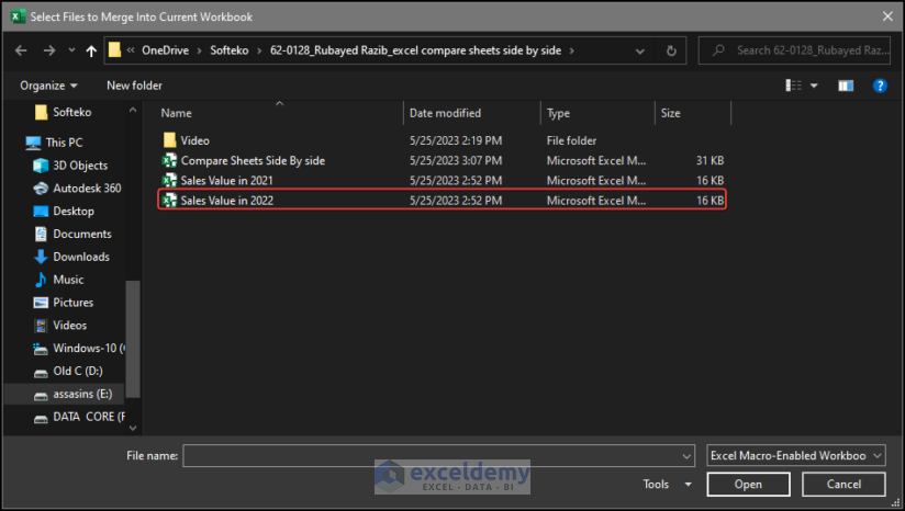
Then a file manager window opens, and from there, choose the second file with which you want to compare the first file.
Click Open.

After clicking Open, we can see that the values in the first file that are not matched with the second file are now highlighted and merged.

4. Using Excel Inquire Add-ins to Compare Sheets Side by Side in Excel

Add-ins are an important part of the Excel ecosystem. With the help of Add-ins, we can carry out complicated operations and tasks. We are going to add the COM Add-ins in this case.

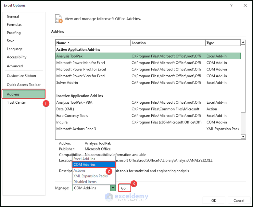
First, go to Files > Options.

Then from the options window, go to Add-ins > COM Add-ins > Go to.

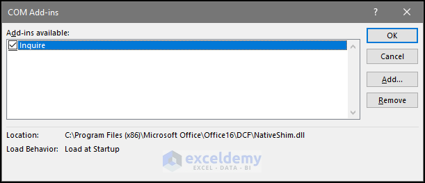
You will see the Inquire check box in the COM Add-ins, check that box and then click on the OK button.

Then in the ribbon menu, click on the Inquire tab, and then click on Compare Files command.

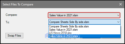
After that, there will be another box asking which files are going to be compared with which files.
In the First row, we already see the parent workbook name in which we are doing this process.
Then we will select the second file in the To drop-down box.

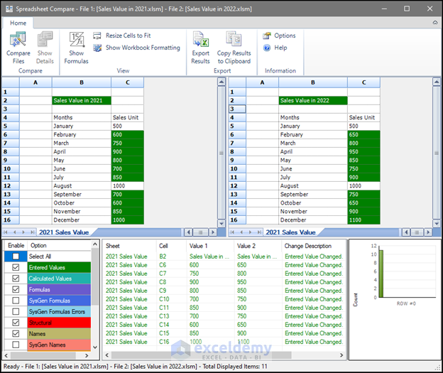
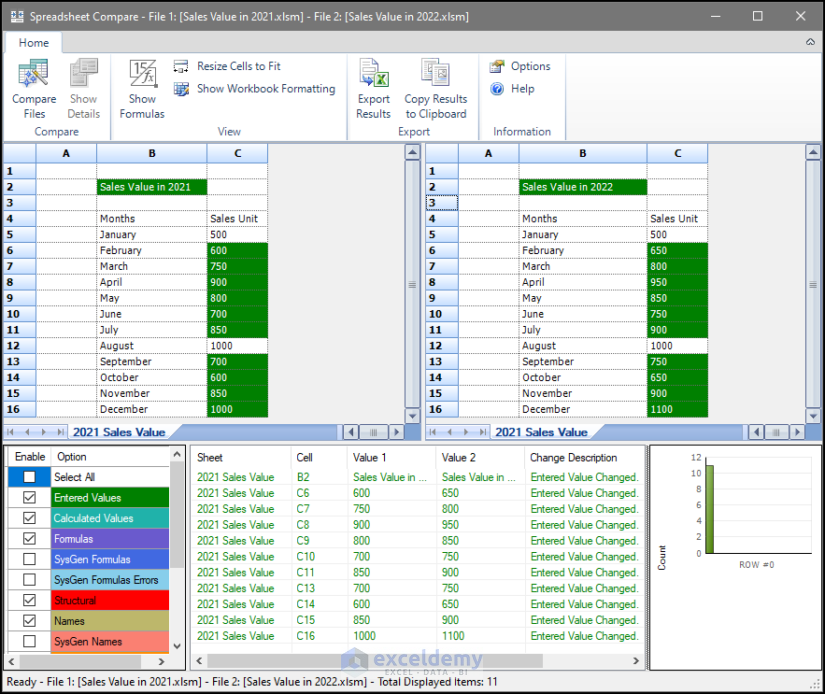
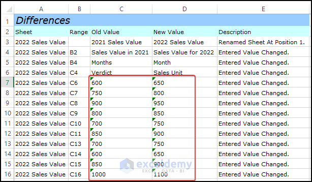
Then in a spreadsheet window, we can see that both of the spreadsheet’s values are compared side by side, and different values are now highlighted in green
In the below sub-window, we can also see the verdict made on them.

Note: Files to be compared must be kept open while running the Inquire tool.

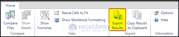
We can also export the comparison in Excel format by clicking on the Export Results

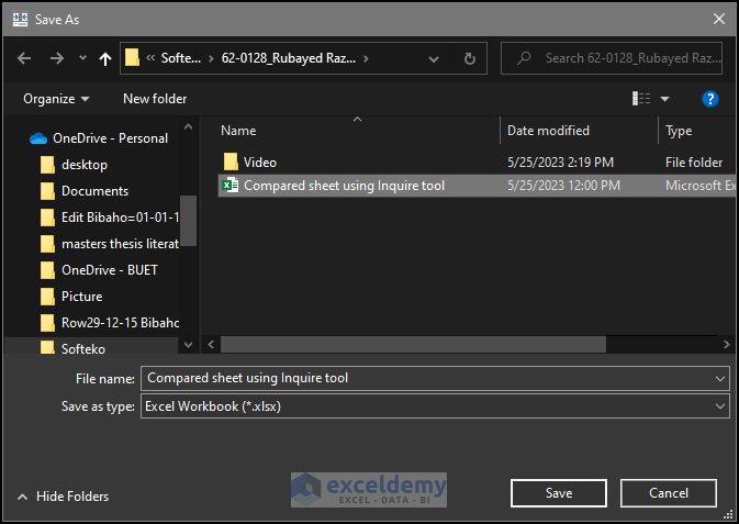
There will be a file manager window that will appear, and the user needs to select the desired location of the file.
Click Save after this.

After selecting Save, we can see that the file is now saved in the desired location.
Then, after opening the file, we can see a new worksheet showing the difference in values highlighted in red.

5. Using VBA Code to Compare Sheets Side by Side in Excel

In addition to the other methods described above, we can get the differences between the values using the VBA methods.

For this, you need to open the VBA editor following the article given here.
Then in the code editor, paste the code given below,

Sub Comparison_of_Worksheet()
    Dim wrkbk1 As Workbook, wrkbk2 As Workbook, wb3 As Workbook
    Dim ws1 As Worksheet, ws2 As Worksheet, ws3 As Worksheet
    Dim lstRw As Long, i As Long
    Dim cell1 As Range, cell2 As Range
    Set wrkbk1 = Workbooks.Open("E:\Onedrive - Softeko\OneDrive\Softeko\62-0128_Rubayed Razib_excel compare sheets side by side\Sales Value in 2021")
    Set wrkbk2 = Workbooks.Open("E:\Onedrive - Softeko\OneDrive\Softeko\62-0128_Rubayed Razib_excel compare sheets side by side\Sales Value in 2022")
    Set wb3 = ThisWorkbook
    Set ws1 = wrkbk1.Sheets("2021 Sales Value")
    Set ws2 = wrkbk2.Sheets("2022 Sales Value")
    Set ws3 = wb3.Sheets("Comparison")
    lstRw = ws1.Cells(ws1.Rows.Count, "B").End(xlUp).Row
    For i = 5 To lstRw
        Set cell1 = ws1.Cells(i, "C")
        Set cell2 = ws2.Cells(i, "C")
        Debug.Print ws1.Cells(i, "C")
        Debug.Print ws2.Cells(i, "C")
        If cell1.Value = cell2.Value Then
            ws3.Cells(i, "C").Value = "Value matched"
        Else
            ws3.Cells(i, "C").Value = "Not matched"
        End If
    Next i
    wrkbk1.Close False
    wrkbk2.Close False
    MsgBox "Comparison completed. Results are listed in the third workbook."
End Sub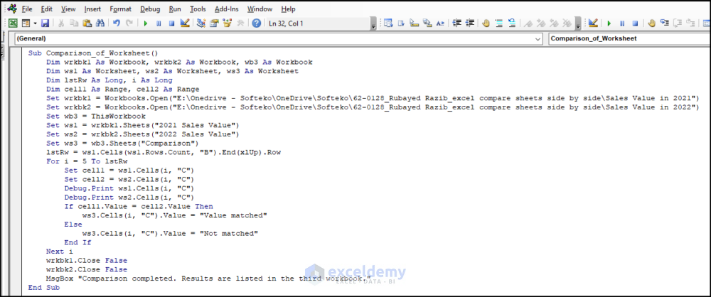

VBA Code Breakdown

Sub Comparison_of_Worksheet()

This line defines the start of the VBA subroutine (macro) named “Comparison_of_Worksheet”.

    Dim wrkbk1 As Workbook, wrkbk2 As Workbook, wb3 As Workbook

This line declares three variables: wrkbk1, wrkbk2, and wb3, all of the Workbook types. These variables will represent the workbooks that will be opened and used for comparison.

    Dim ws1 As Worksheet, ws2 As Worksheet, ws3 As Worksheet

This line declares three variables: ws1, ws2, and ws3, all of the Worksheet types. These variables will represent the worksheets within the workbooks that will be used for comparison.

    Dim lstRw As Long, i As Long

This line declares two variables: lstRw and i, both of the Long data types. lstRw will store the last row number in the worksheet, and I will be used as a loop counter.

    Dim cell1 As Range, cell2 As Range

This line declares two variables: cell1 and cell2, both of the Range data type. These variables will represent specific cells in the worksheets for comparison.

    Set wrkbk1 = Workbooks.Open("E:\Onedrive - Softeko\OneDrive\Softeko\62-0128_Rubayed Razib_excel compare sheets side by side\Sales Value in 2021")
    Set wrkbk2 = Workbooks.Open("E:\Onedrive - Softeko\OneDrive\Softeko\62-0128_Rubayed Razib_excel compare sheets side by side\Sales Value in 2022")

These two lines open two workbooks (“Sales Value in 2021” and “Sales Value in 2022”) and assign them to the wrkbk1 and wrkbk2 variables, respectively

    Set wb3 = ThisWorkbook

This line assigns the workbook containing the VBA code (the workbook where the macro is stored) to the wb3 variable.

    Set ws1 = wrkbk1.Sheets("2021 Sales Value")
    Set ws2 = wrkbk2.Sheets("2022 Sales Value")
    Set ws3 = wb3.Sheets("Comparison")

These three lines assign specific worksheets within the workbooks to the ws1, ws2, and ws3 variables, respectively. These worksheets will be used for comparison and result display.

    lstRw = ws1.Cells(ws1.Rows.Count, "B").End(xlUp).Row

This line determines the last row in the ws1 worksheet by finding the last non-empty cell in column B.

    For i = 5 To lstRw

This line starts a loop that will iterate from row 5 to the last row in the ws1 worksheet.

        Set cell1 = ws1.Cells(i, "C")
        Set cell2 = ws2.Cells(i, "C")

These two lines assign the cells in column C for the current row (i) in ws1 and ws2 to the cell1 and cell2 variables, respectively.

        Debug.Print ws1.Cells(i, "C")
        Debug.Print ws2.Cells(i, "C")

These two lines print the values of cell1 and cell2 (for debugging purposes).

        If cell1.Value = cell2.Value Then
            ws3.Cells(i, "C").Value = "Value matched"
        Else
            ws3.Cells(i, "C").Value = "Not matched"
        End If

This block of code compares the values of cell1 and cell2. If they are equal, the corresponding cell in the ws3 worksheet is set to “Value matched”. Otherwise, it is set to “Not matched”.

    Next i

This line indicates the end of the loop and moves to the next iteration.

    wrkbk1.Close False
    wrkbk2.Close False

These two lines close the wrkbk1 and wrkbk2 workbooks without saving any changes.

    MsgBox "Comparison completed. Results are listed in the third workbook."

This line displays a message box with the specified message, indicating that the comparison is completed and the results can be found in the third workbook.

End Sub

This line marks the end of the VBA subroutine.

After pressing the Run command, we can see that the comparison between the worksheet from different workbooks has been made, and the verdict is made in the range of cells C5:C16.

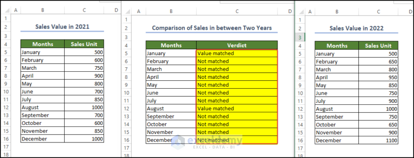
Note: You need to close the file before running the code, otherwise, it can show errors.

Things to Remember

Open/Close both sheets: Open the two Excel sheets that you want to compare. You can open them in separate windows or arrange them in split view within the same Excel window. Or you may need to close both sheets in different cases before starting to compare them.

Arrange windows: If you have opened the sheets in separate windows, arrange the windows side by side on your computer screen. You can do this by manually resizing and positioning the windows or by using the “Arrange All” feature in Excel.

Lock headings: If your sheets have headings or column labels, it can be helpful to lock them in place so that they remain visible while scrolling through the data. To do this, select the row containing the headings, right-click, and choose “Freeze Panes” or “Freeze Top Row” from the context menu.

Scroll together: To compare the data in both sheets, make sure that scrolling is synchronized between the two windows. This way, when you scroll vertically or horizontally on one sheet, the other sheet scrolls accordingly. Some versions of Excel provide a “Synchronous Scrolling” option in the “View” tab or a similar feature to enable this.

Highlight differences: To easily spot differences between the two sheets, you can use conditional formatting. Select the range of cells you want to compare, go to the “Home” tab, click on “Conditional Formatting,” and choose the desired rule to highlight the differences. For example, you can highlight cells that are not equal or cells with unique values.

Use formula-based comparisons: Excel provides various functions that can help you compare data between sheets. Functions like VLOOKUP, INDEX–MATCH, or IF can be used to retrieve information from one sheet based on values in another sheet, allowing you to identify matching or mismatched data.

Take notes: If you need to make observations or document the differences you find, consider having a separate sheet or document open where you can take notes while comparing the sheets side by side. This can be helpful for future reference or when discussing the findings with others.

Frequently Asked Questions

1. Can you use VLOOKUP to compare two spreadsheets?

You can use the VLOOKUP function to compare sheets side by side using the following formula stated below,

=VLOOKUP(C5,'[Sales Value in 2022.xlsm]2022 Sales Value'!$C$4:$C$15,1,FALSE)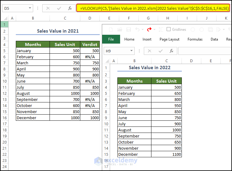

We compared the values in 2021 with the values in 2022. If the match values are found, then the value will stay in place. Otherwise, N/A will be shown in the cell.
In this way, you can compare sheets side by side.

2. How to compare two columns in different Excel sheets using if?

You can use the below formula to compare the values of a cell from one parent sheet to another.

=IF(C5='E:\Onedrive - Softeko\OneDrive\Softeko\62-0128_Rubayed Razib_excel compare sheets side by side\[Sales Value in 2022.xlsm]2022 Sales Value'!C4, "Match", "Value Not Matched")

Here in the formula, we can see that the user compared cell C5 with another sheet in a separate workbook and show whether they matched or not.

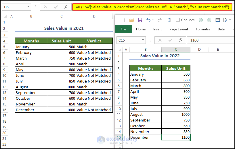
If the cell values matched, the “Match” will be written on the side. Or “ Value Not Matched”.

3. How to compare two columns in different Excel sheets for matches?

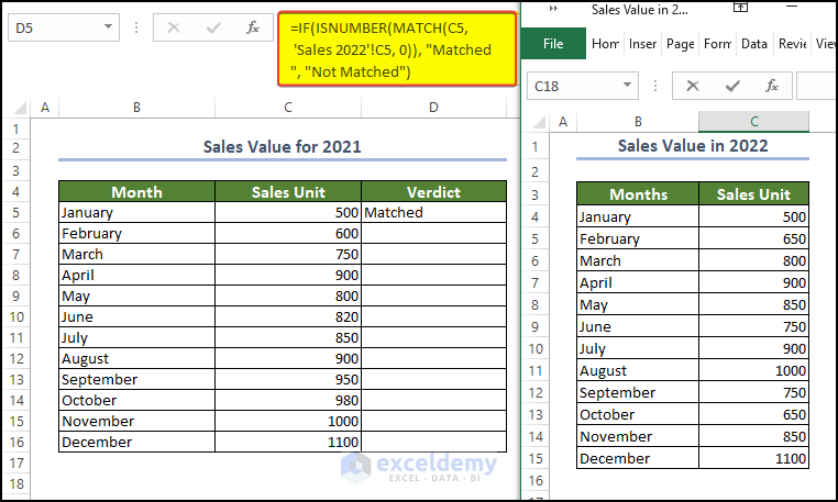
With the combination of the IF, ISNUMBER, and MATCH functions, we can compare two columns in different Excel sheets

You can use the below formula to compare the values of a cell from one parent sheet to another.

=IF(ISNUMBER(MATCH(A1, Sheet2!A:A, 0)), A1, "")

Here, the A1 denotes the values in the parent sheet cell value, and this will search for this cell value in column A in Sheet 2. If there are any matched values, then that value will be placed in the A1 cell. If there is no match, the cell will be empty.

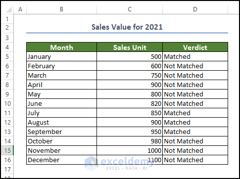
After dragging the fill handle to cell D16.
After dragging the fill handle to cell D16, we will see that the range of cell D5:D16 is now filled with the verdict whether they are matched with other sheet values or not.

Download Practice Workbooks

Download the following workbook to practice by yourself.

Comparing Sheets Side by Side.xlsm

Sales Value in 2021.xlsm

Sales Value in 2022.xlsm

Compared sheet using Inquire tool.xlsm

<< Go Back to Learn Excel | Compare | Worksheets

Conclusion

In this article, we have shown how, in Excel, we can compare multiple sheets side by side. The methods included VBA macro, Side by Side view window, Compare and Merge, using the Inquire tool, etc. Which method a user wants to use completely depends on the user’s choice and their own problem statement. Feel free to comment anything, we will reply to that as early as possible.