In this article, we will demonstrate how to fix the Excel circular reference that cannot be listed in Excel. It’s very intimidating if you get circular reference errors while working on Excel. While working on a large dataset that contains thousands of cells it can be very difficult to identify the cells that contain circular reference errors by checking each cell one by one. So, in this tutorial, we will explain how we can list circular reference errors easily from any size of the dataset.
What is Circular Reference?
A circular reference is a formula that returns the same or another cell numerous times in its sequence of calculations, resulting in an infinite loop that severely slows down your spreadsheet.
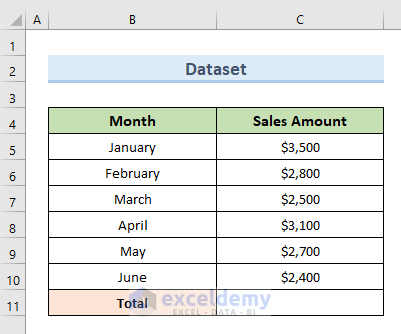
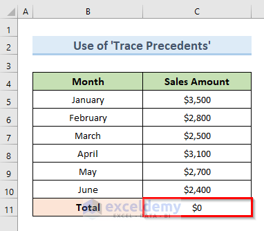
To illustrate circular reference more clearly we will use the following dataset. The dataset consists of “Sales Amount” for six months. Suppose, we need to calculate the total amount of sales in cell C11.
Now, we have to select the cell range (C6:C10) in the SUM function to get the result. If we accidentally select the cell range (C6:C11) you might not get the result that you are expecting.
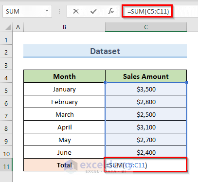
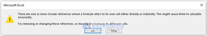
The above formula in cell C11 gives us a warning of circular reference error. This happens because the formula in cell C11 is trying to enumerate itself too.
We can categorize circular reference errors into two types:
1. Direct Circular Reference:
A direct circular reference error shows up when a formula in a cell directly refers to its cell.
2. Indirect Circular Reference:
An indirect circular reference occurs when a formula in a cell doesn’t refer to its cell directly.
How to Fix Excel Circular Reference That Cannot be Listed: 4 Easy Ways
When we get a circular reference error at the time of calculation we must fix that or immediately. To fix that error first, we need to locate them. So, in this article, we will use 4 different methods to list the circular reference error, and then we will fix the errors by modifying the formula.
1. Fix Circular References That Cannot be Listed with Error Checking Tool in Excel Ribbon
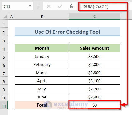
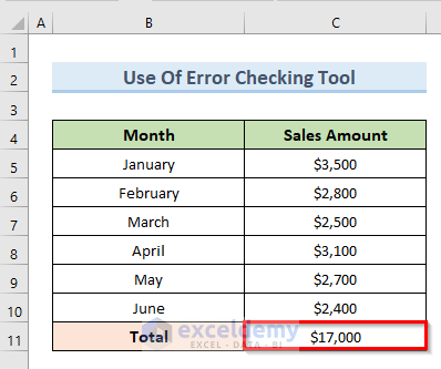
First and foremost, will use the ‘Error Checking’ tool from the Excel ribbon to identify the circular reference errors that cannot be listed. To explain this method we will use the following dataset that contains a circular reference error in cell C11. The following dataset is just an example to make you understand better. When you work with a real-time dataset you have to find out circular references from thousands of cells.
Let’s see the steps to list circular reference errors by using the ‘Error Checking’ tool.
STEPS:
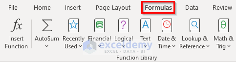
- Firstly, go to the Formulas tab.
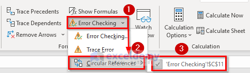
- Secondly, from the Excel ribbon under the Formulas tab select the drop-down “Error Checking”. From the drop-down menu click on the option “Circular References”.
- The above action is showing in a sidebar that circular reference is happening at cell C11 in our worksheet.
- In short: Go to Formulas > Error Checking > Circular References > ‘Error Checking’!$C$11.
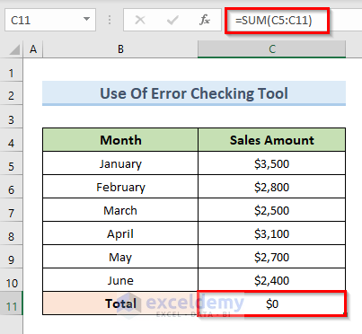
- Thirdly, select cell C11. The formula in that cell is trying to calculate itself too.
- After, that modify the formula of cell C11 like the following one:
=SUM(C5:C10)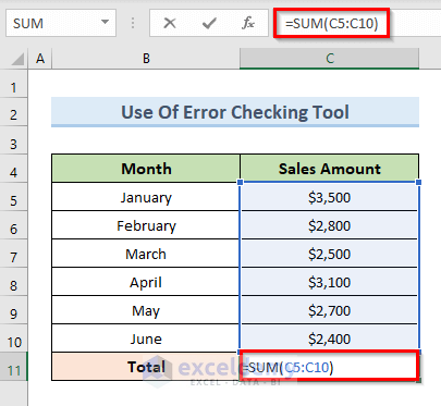
- Press Enter.
- Lastly, we can see that there is no circular reference error in cell C11. So, the amount of total sales in cell C11 is $17000.
Read More: How to Fix Circular Reference Error in Excel
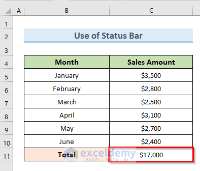
2. Use Status Bar to Fix Circular References in Excel That Cannot be Listed
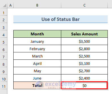
Finding circular reference errors by using the “Status Bar” is the easiest way. To explain the process of how to list the Excel circular reference that cannot be listed with the “Status Bar” we will continue with the same dataset that we used in the previous example.
Let’s see the steps to list and fix circular references with the “Status Bar”.
STEPS:
- First, open the worksheet that contains circular reference errors.
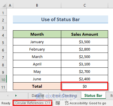
- Next, look at the “Status Bar” below the worksheet names.
- From the “Status Bar”, we can see that there is a circular reference error in cell C11.
- After that, modify the formula of cell C11 by changing the range from (C5:C11) to (C5:C10).
=SUM(C5:C10)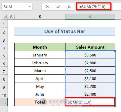
- Press Enter.
- Finally, the above commands fix the circular reference error in cell C11 and return the total amount of cells.
NOTE:
If any worksheet has two or more cells that contain circular references the “Status Bar” will only show the latest one.
Read More: [Fixed!] Iterative Calculation Not Working in Excel
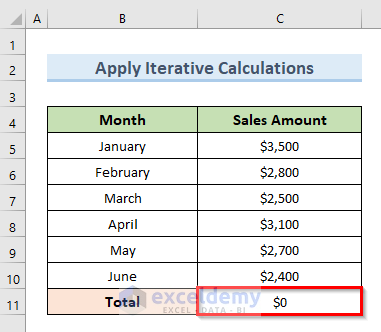
3. Apply Iterative Calculation to Fix Circular References in Excel
We can also fix the Excel circular reference that cannot be listed from our worksheet by using iterative calculations. We can list and fix the circular references in our worksheet by enabling iterative calculation in our Excel worksheet. To illustrate this method will use the dataset of our previous example this time also.
Let’s take a look at the steps to perform this action.
STEPS:
- In the beginning, go to the File tab.
- Next, select Options.
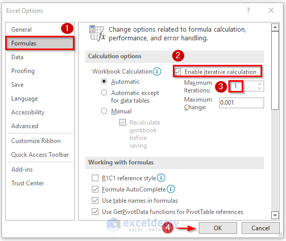
- Then, a new dialogue box named “Excel Options” will appear.
- From that box select Formulas and check the option “Enable iterative calculation”. Set the value 1 for “Maximum iterations”. The value 1 indicates that the formula will iterate only once through the cells C5 to C10.
- Now, press OK.
- Finally, we do not get any circular reference errors in cell C11. It returns the total sales amount in cell C11.

Read More: Enable Iterative Calculation in Excel
4. Find & Fix Circular References in Excel with Tracing Methods
We can not find and fix circular references with a single click. To fix the Excel circular reference that cannot be listed we will trace them one by one. After tracing we will modify their initial formula to fix the circular reference errors. The tracing methods we will use in this section are “Trace Precedents” and “Trace Dependents”.
4.1 ‘Trace Precedents’ Feature to Fix Circular Reference
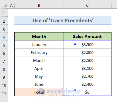
The “Trace Precedents” feature traces the cells that are dependent on the current cell. This feature will tell us which cells are affecting the active cell by drawing an arrow line. In the following dataset, we will return the sum of cell cells (C5:C10) in cell C11. So, cell (C5:C10) is affecting cell C11.
So, let’s see the use of “Trace Precedent” step-by-step.
STEP:
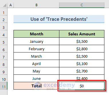
- Firstly, select cell C11.
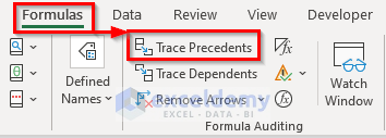
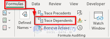
- Secondly, go to the Formulas tab.
- Then, select the option “Trace Precedents”.
- The above action draws an arrow line. It shows that cells (C5:C11) are affecting Cell C11. As cell C11 is trying to enumerate itself so it returns a circular reference error.
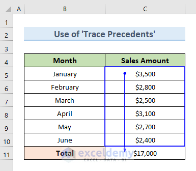
- Thirdly, modify the formula of cell C11 by changing the range in the formula to (C5:C10) from (C5:C11). The formula in cell C11 will be:
=SUM(C5:C10)
- After that, press Enter. The above command removes the circular reference from that cell.
- Finally, use the “Trace Precedents” option in cell C11 We will see that this time cells (C5:C10) are affecting cell C11 whereas in the previous step the cells affecting cell C11 were (C5:C11).
NOTE:
The keyboard shortcut to find Trace Precedents: ‘Alt + T U T’.
4.2 ‘Trace Dependents’ Feature to Fix Circular Reference
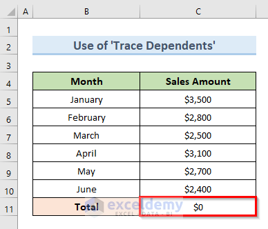
The “Trace Dependents” feature is used to find the cells that are dependent on the active cell. The feature will show us the cells that depend on the active cell by drawing a line arrow. In the following dataset, we will list circular reference errors with the “Trace Dependents” option.
So, let’s take a look at the steps to list circular references by using the “Trace Dependents” option.
STEPS:
- First, select cell C11.
- Next, go to the Formulas tab.
- Select the option “Trace Dependents” from the ribbon.
- Then, the above action shows that cells (C5:C10) are depending on cell C11 by drawing a line arrow.

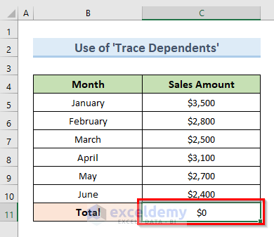
- After that, adjust the formula of cell C11 by changing the range in the formula to (C5:C10) from (C5:C11). The formula in cell C11 will be:
=SUM(C5:C10)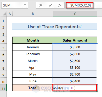
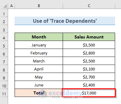
- Press Enter.
- Lastly, we can see that there is no circular reference in cell C11.
NOTE:
The keyboard shortcut to find Trace Precedents: ‘Alt + T U D’.
Read More: How to Find a Circular Reference in Excel
Download Practice Workbook
You can download the practice workbook from here.
Conclusion
In the end, this tutorial will show you how to fix Excel circular references that cannot be listed. Use the practice worksheet that comes with this article to put your skills to the test. If you have any queries, please leave a comment below.
Related Articles
<< Go Back to Circular Reference | Cell Reference in Excel | Excel Formulas | Learn Excel
Get FREE Advanced Excel Exercises with Solutions!
