What is A Circular Reference?
A circular reference occurs when a formula, either directly or indirectly, refers back to its cell reference, resulting in an unending loop of computations.
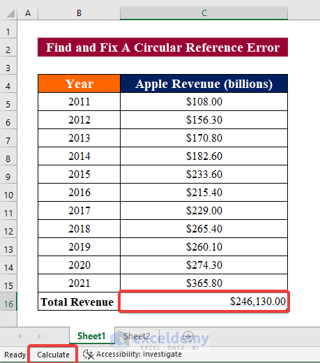
Here’s an example :
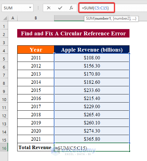
The SUM Function is used in C16 to compute the total revenue. However, C5:C16 is declared as range in the SUM Function.
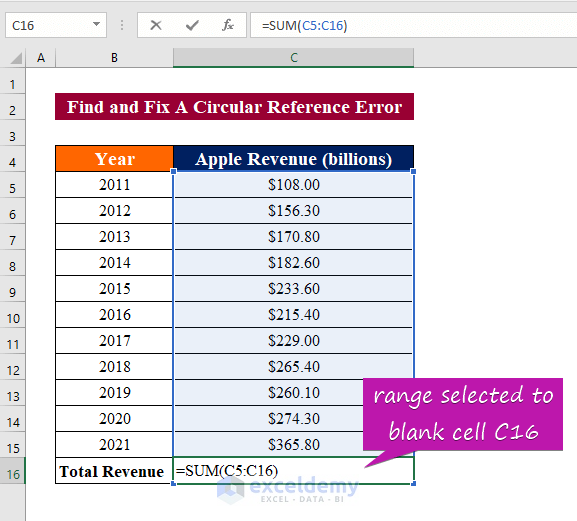
It creates an endless loop and Excel will keep adding the new value to C16.
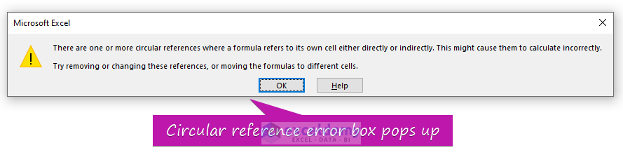
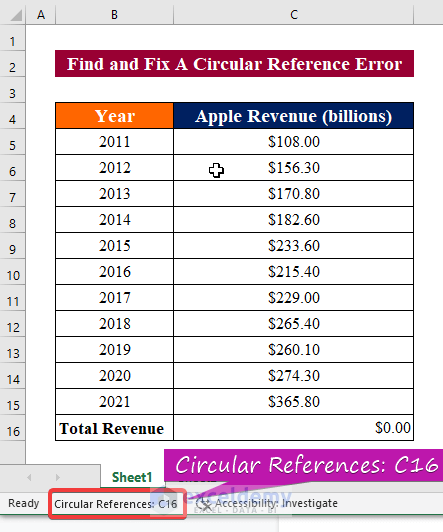
A circular reference warning is displayed:
Use Iterative Calculations to Enable/Disable the Circular Reference Error
Enable/Disable Iterative Calculations
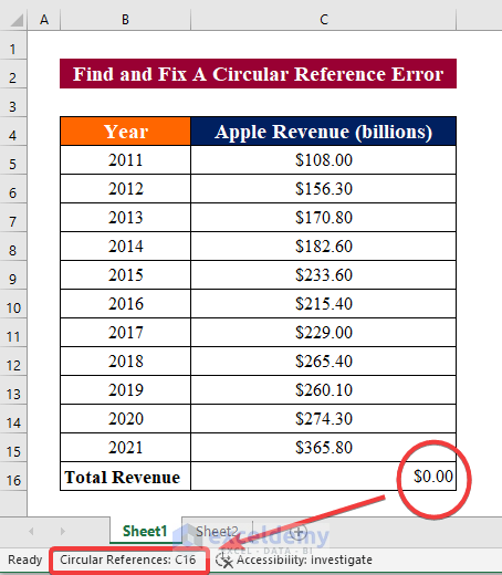
In the image below, a circular reference in C16 is indicated in the status bar. The result is zero (0) in C16. To enable Iterative calculations:
Steps:
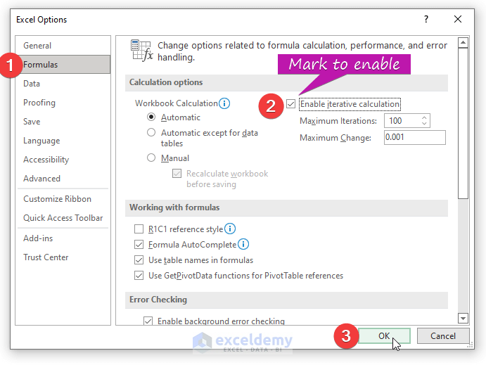
- Go to the File tab ⇨ Options ⇨ Formulas.
- Check Enable iterative calculation.
- Press Enter.
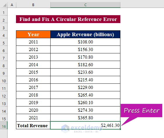
This is the output.
Each cell related with the circular reference will be calculated.
Maximum Iterations & Maximum Change Parameters
Iterative Calculations have two parameters:
Maximum Iterations
The loop is repeated when Excel calculates the final result.
Maximum Change
The number that must be achieved in order that the iteration will continue. By default, the maximum change is set to 0.001.
Why Should Enabling Iterative Calculations be avoided?
When you enable iterative calculations, the deliberate usage of circular references uses resources and computing power and may result in unwanted or inaccurate consequences.
Finding a Circular Reference Error in Excel
1. Use the Error Checking Feature to Find a Circular Reference Error in Excel
Step 1:
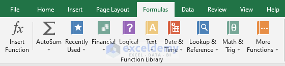
- Go to the Formulas tab
- Click Error Checking.
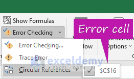
Step 2:
- Select Circular References.
Excel will display all circular references in the worksheet.
Read More: How to Find a Circular Reference in Excel
2. Use the Status Bar to Find a Circular Reference Error in Excel
If the worksheet has a circular reference, it is displayed in the status bar below the worksheet names.
Note.
- This feature is disabled when the Iterative Calculation option is enabled.
- It only displays the most recent circular reference.
Read More: How to Allow Circular Reference in Excel
Fix a Circular Reference Error in Excel
Step 1:
- Select the correct range to fix the error in C16.
Step 2:
- Press Enter in C16 to see the result.
Read More: How to Remove Circular Reference in Excel
Trace Relationships Between Formulas and Cells
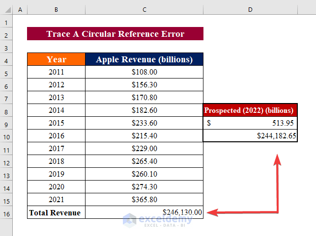
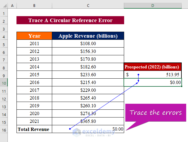
The dataset below showcases the prospected revenue of Apple in 2022. To Sum the total revenue from 2011 to 2022, the following formula was used in D10.
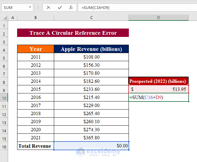
As there is a circular reference in C16, there will be an error in D10.
Trace Precedents to Relate a Circular Reference Error in Excel
Steps:
- Go to the Formulas tab.
- Select Trace Precedents.
 You will see arrows that indicate cells that affect the active ones.
Note. The shortcut to Trace Precedents is Alt+T U T
Trace Dependents to Relate a Circular Reference Error in Excel
Steps:
- Go to the Formulas tab.
- Select Trace Dependents.
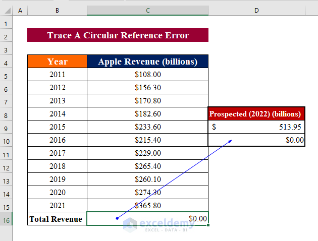
 Cells containing formulas that refer to the active cell are displayed.
Note. The shortcut to Trace Dependents is Alt+T U D
Download Practice Workbook
Download the practice workbook.
Related Article
<< Go Back to Circular Reference | Cell Reference in Excel | Excel Formulas | Learn Excel
Get FREE Advanced Excel Exercises with Solutions!
