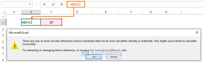
“Allow Circular Reference in Excel” is an easy way to insert self-reference a cell in Excel. By Microsoft’s definition, Circular Reference occurs when an Excel formula refers back to its own cell, either directly or indirectly. For example, if we want to add two entries (i.e., B2 and C2) but display the result in one of the entries (i.e., B2), then we create a circular reference. After hitting ENTER for the first time Excel shows a warning that there are one or more circular references in the formula only.
Circular reference calculates formula results in iterations. As a result, it can create a loop if the maximum iteration time is set too much.
In this article, we discuss circular reference, its issues, and its usage.
How to Find Circular Reference is Enabled or Not?
From the previous sections, we know what circular reference is and how to deal with it. Though the most relevant question is how to find whether an Excel worksheet has circular reference Enabled or Disabled?
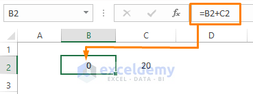
The most natural way is that if we enter references by ourselves, Excel shows a warning for the first time as shown in the following image. If Excel displays the warning, we are pretty sure that the worksheet has circular reference disabled. Otherwise, the formula returns the correct result for the maximum iterative number 1.
After entering cell references in formulas, you see Excel returns zero (0) without any obvious reasons. You check the text to the right side of the Ready status at the bottom of any worksheet. If it shows Circular Reference: cell, the circular reference option is disabled for the worksheet.

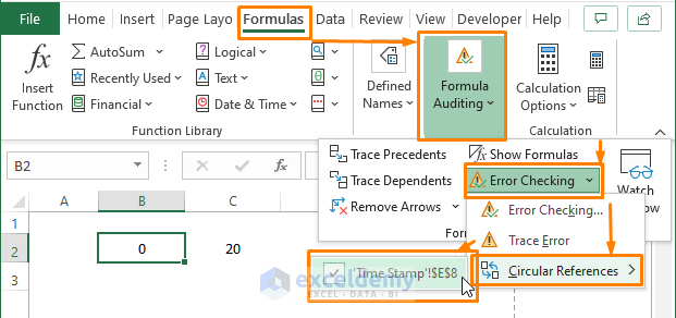
We can go to the Formulas Tab > Select Error Checking (in the Formula Auditing section) > Select Circular References (from the Error Checking options). It shows where the error of the circular reference takes place.
Allow Circular Reference in Excel Using the File Ribbon
Allowing circular reference is one kind of ignoring a reference error in formulas. Nevertheless, allowing circular reference enables formulas to overcome reference error and return the correct resultant value.
In order to allow circular reference, Follow the below sequences,
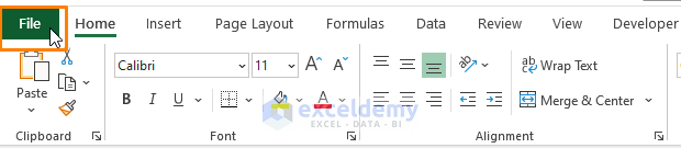
➤ Go to the File Ribbon of any worksheet.
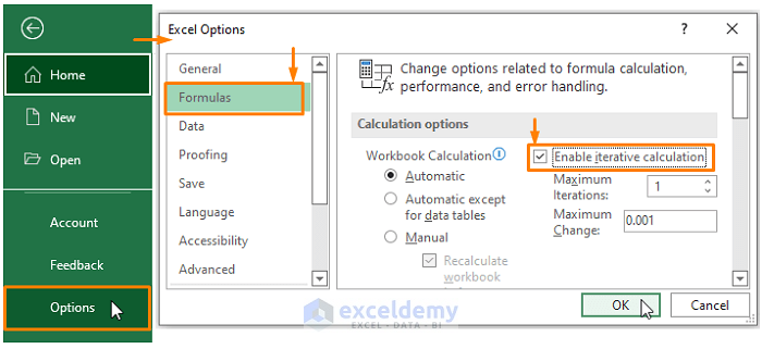
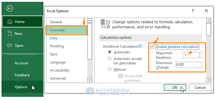
➤ Select Options from the File menu options (the Excel Options window appears) > Select Formulas (in the right side of the window) > Tick the Enable iterative calculation option (entering your needed Maximum iterations number and Maximum change).
Click OK.
 Executing these sequences, you can allow formulas to return resultant values with existing Circular References.
Read More: How to Fix Circular Reference Error in Excel
Issues with Maximum Iterations
When a circular reference occurs in Excel, Excel returns a warning for the first time as shown in the below screenshot.

However, later on, Excel doesn’t show the warning, and users are stuck on calculations wondering what goes wrong as resultant values return zero (0) irrespective of formula types.
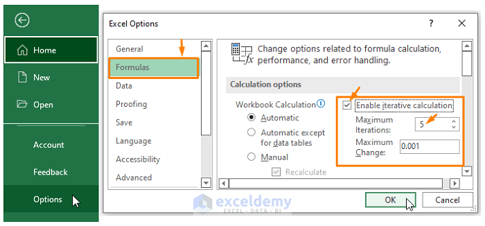
To solve this calculation issue, we have to check the enable iterative calculation option. Go to the File Tab option as instructed in the following image.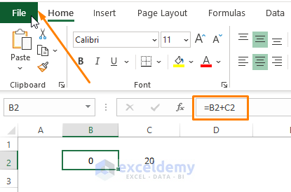
After clicking on File Ribbon, Select Options (the Excel Options window appears) > Choose Formulas (in the left section of the Excel Options window) > Tick the Enable iterative calculation. Then click OK.
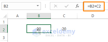
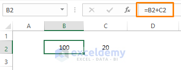
 Now, we can use circular references in formulas. But if you enter 1 (as we entered) in the Maximum iterations box the formula (i.e.,
 =B2+C2) returns 20 (which is correct as B2 is empty and C2 has a value of 20) as depicted in the below image.
However, if we enter 5 in the Maximum iterations option box, as we are displaying in the following screenshot.
The formula returns 100 as it iterates the same calculation 5 times. It’s the most disturbing miscalculation in Excel.
Read More: [Fixed!] Iterative Calculation Not Working in Excel
Uses of Circular Reference in Excel: 2 Examples
Circular Reference is quite useful in certain areas. Some incidents need Circular Reference to represent values more effectively. In this article, we discuss two of the most used Circular Reference instances.
Example 1: Allow Circular Reference in Excel to Insert Static Timestamp
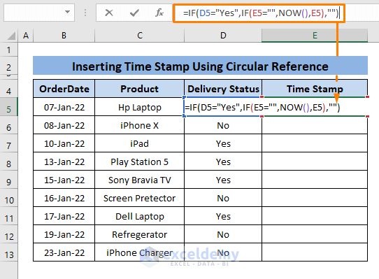
Let’s say we have some Products with Order Dates and Delivery status. And we want to insert a Timestamp in cells whatever the Products are delivered. We show Delivery Status in Yes or No’s.
So, if the Delivery Status is Yes then the Timestamp displays the then Time and Date.
➤ Paste the following formula in any blank cell (i.e., E5) where you want to display the Timestamp.
=IF(D5="Yes",IF(E5="",NOW(),E5),"")The formula runs a logical_test to match Yes with entries in column D. Then it displays the current time in cells that return TRUE or keep the cell blank otherwise.
➤ Press ENTER then Drag the Fill Handle to insert the Timestamp to all delivered products.
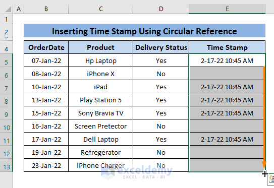
Since Circular Reference poses a self-cell reference issue, sometimes it seems the formula might not work properly. In that case, rewrite the Delivery Status or conditions then apply any formulas. And you may need to change the cell format to get the date-time format.
Read More: Fix Circular Reference That Cannot be Listed in Excel
Example 2: Allow Circular Reference in Excel for Iterative Calculation
Sometimes, we need to perform iterative calculations. In an iterative calculation, we get the direct iterative value without performing the whole calculation.
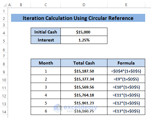
Suppose in a scenario, we invest an initial cash amount (i.e., $1500) and we want monthly installments from the asset. We can calculate the installment amounts for the 1st month using the below formula.
=$C$4*(1+$C$5)Then refer to the previous installment amount to calculate the next installment amounts as shown in the following picture.
➤ However, if we use circular reference, we can get the nth installment amount just by entering the installment number as the Maximum iterations number. For the correct result, we enter 5 as Maximum iterations and the 1th of 1000 allowable changes as shown in the image below.
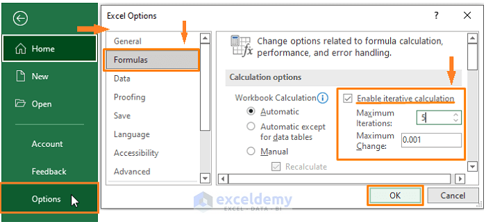 We enter the maximum iterations number 5 because we have to calculate the 6th installment. And we allow the changeable amount to vary 1th of 1000 portions.
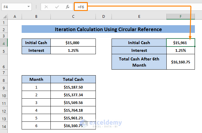
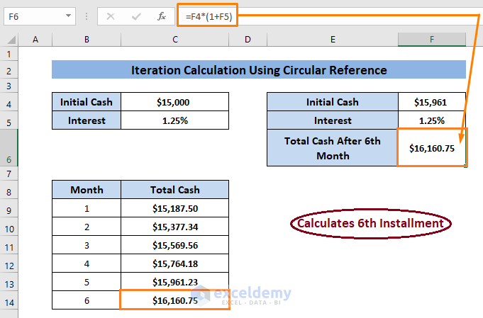
➤ After allowing Circular Reference, Type =F6 in cell F4 to fetch the calculated value after 5th iterations in cell F6 (creating Circular Reference) applying =F4*(1+F5) formula.
The formula in the F6 cell calculates the 6th installment in the second and enduring less hassle.
Download Excel Workbook
Conclusion
In this article, we discuss one of Excel’s most annoying incidents, Circular Reference. Also, we look after issues created by the Maximum iterations option. We demonstrate the common usage of Circular Reference and tricks to use it in suitable calculations. Hope this article clarifies your concept regarding Circular Reference and helps you to handle it more effectively. Comment if you have further queries or anything to add. See you in my next article.
Related Articles
<< Go Back to Circular Reference | Cell Reference in Excel | Excel Formulas | Learn Excel
Get FREE Advanced Excel Exercises with Solutions!
