A credit card can be a blessing or a curse. It all depends on a person’s financial knowledge. This article will show you quick steps to create a credit card payoff calculator with amortization in Excel. We will also insert an Excel VBA Macro to hide unnecessary data.
Create Credit Card Payoff Calculator with Amortization in Excel: with Easy Steps
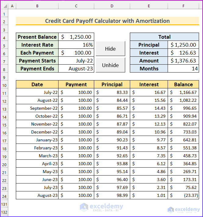
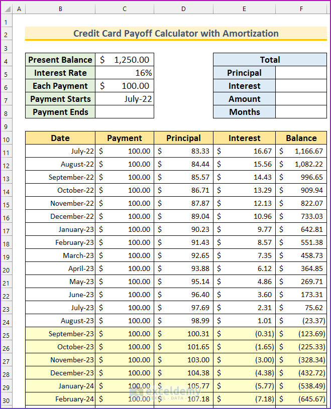
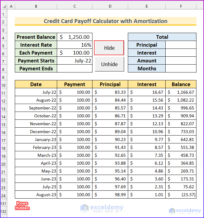
Here is a quick look at the credit card payoff calculator with amortization, which we will create by the end of this tutorial.
Step 1: Setting up the Essentials
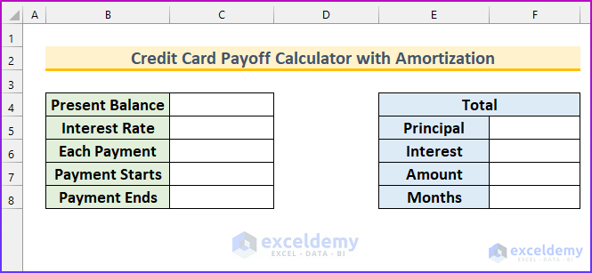
In this first step, we will create the fields where the basic info about the debt will be inserted.
- Firstly, type the following fields related to the credit card payoff:
- Present Balance
- Interest Rate
- Each Payment
- Payment Starts
- Payment Ends
- Secondly, type these things under the Total field which we will find at the last step of this article.
- Principal
- Interest
- Amount
- Months
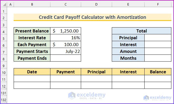
- Thirdly, type the details of the first four fields into the calculator.
- Lastly, create the following 5 columns:
- Date
- Payment
- Principal
- Interest
- Balance
Step 2: Calculating Initial Amounts
In the second step, we will calculate the initial amount of the credit card payoff calculator with amortization.
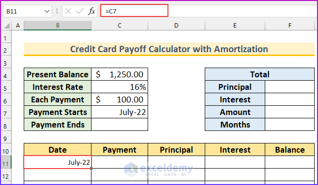
- To begin with, type the following formula in cell B11. This is the first payment date for our credit card debt.
=C7
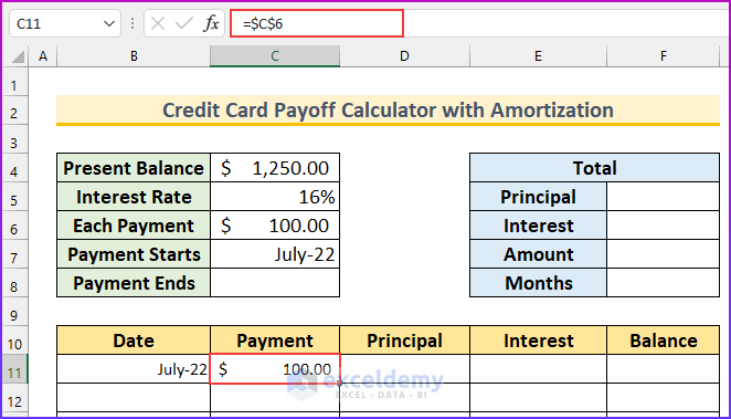
- Next, type another formula to reference the monthly payment in cell C11.
=$C$6
- Then, type a formula in cell E11 to find the amount of interest. We have divided by 12 to find the monthly interest rate from the yearly rate.
=C4*C5/12

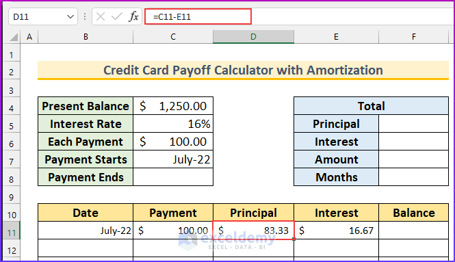
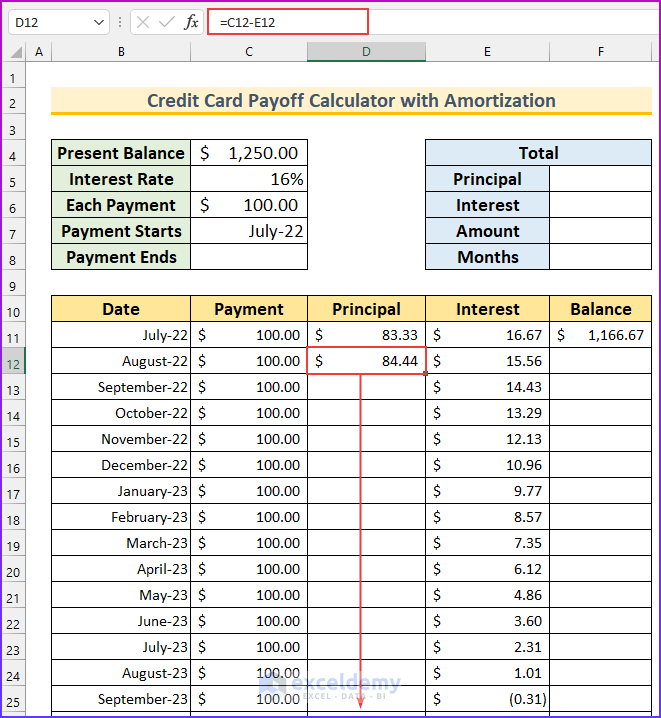
- After that, type this formula in cell D11 to find the principal amount that was paid.
=C11-E11
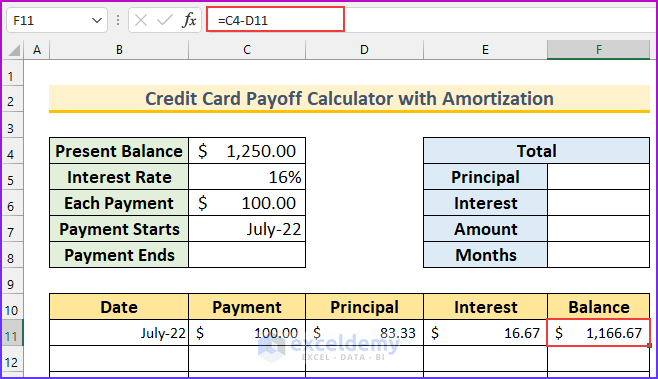
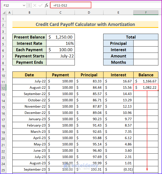
- Lastly, type this formula in cell F11 to find the remaining debts.
=C4-D11
Step 3: Calculating Remaining Amounts
In this step, we will use the DATE, YEAR, MONTH, and DAY functions to display incremental months. Then, we will use simple formulas to find the rest of the amortization amounts.
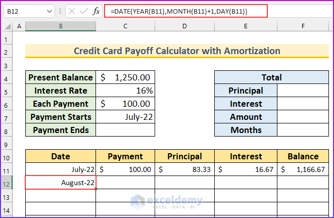
- Firstly, type a formula in cell B12. This formula increases the date by 1 month.
=DATE(YEAR(B11),MONTH(B11)+1,DAY(B11))
- Then, AutoFill the formulas from cells B12 and C11 downward.
- Afterward, type another formula in cell E12. This formula finds the amount of interest on the remaining balance. As before, drag this formula down.
=F11*$C$5/12

- Now, type this formula in cell D12 to find the amount of principal paid. Then, drag the formula downward.
=C12-E12
- Then, type another formula in cell F12 to find the remaining balance and using the Fill Handle, fill in the formula into the rest of the cells.
=F11-D12
- Lastly, we can see that there are more than the necessary rows in the dataset. If our terms are larger, then we don’t need to do anything; it will show up automatically. However, it can be helpful if we hide these rows.
Step 4: Applying VBA to Hide Extra Rows
In this step, we will hide the unnecessary rows using a VBA macro. After that, we will use another code to unhide them. Both of these codes will be applied to two separate VBA buttons.
- To begin with, press ALT+F11 to bring up the VBA module window.
- Next, type this code.
Option Explicit
Sub Hide_Rows()
    Dim Cell_Range As Range
    Application.ScreenUpdating = False
        For Each Cell_Range In Range("E11:E130")
            If Cell_Range.Value < 0 Then
                Cell_Range.EntireRow.Hidden = True
            Else
                Cell_Range.EntireRow.Hidden = False
            End If
        Next Cell_Range
    Application.ScreenUpdating = True
End Sub
Sub Unhide_Rows()
    Rows.EntireRow.Hidden = False
End Sub
VBA Code Breakdown
- We have two Sub procedures in this code.
- The first one hides the rows that have negative values in the cell range E11:E130. Moreover, we are using the For Each Next loop to go through each cell.
- The last one reveals the rows.
- Thus, this code works.
- Then, save and close the Module.
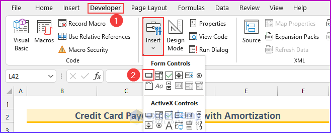
- Now, from the Developer tab → Insert → select Button (Form Control).
- Then, it will change the mouse cursor. Drag a box in the dataset, then upon releasing the mouse the Assign Macro window will appear.
- After that, select “Hide_Rows” and press OK. Then, drag another box and select “Unhide_Rows” from the option and press OK.
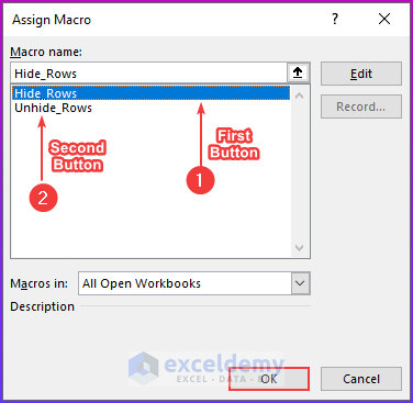
- Then, we renamed the buttons to Hide and Unhide respectively.
- Now, if we click on the “Hide” button it will hide all the extra rows.
Step 5: Finding Total Debt Paid
In the last step, we will finish inputting the values that we left blank in the first step. We will use the INDEX, MATCH, SUM, SUMIF, and COUNTIF functions in this step.
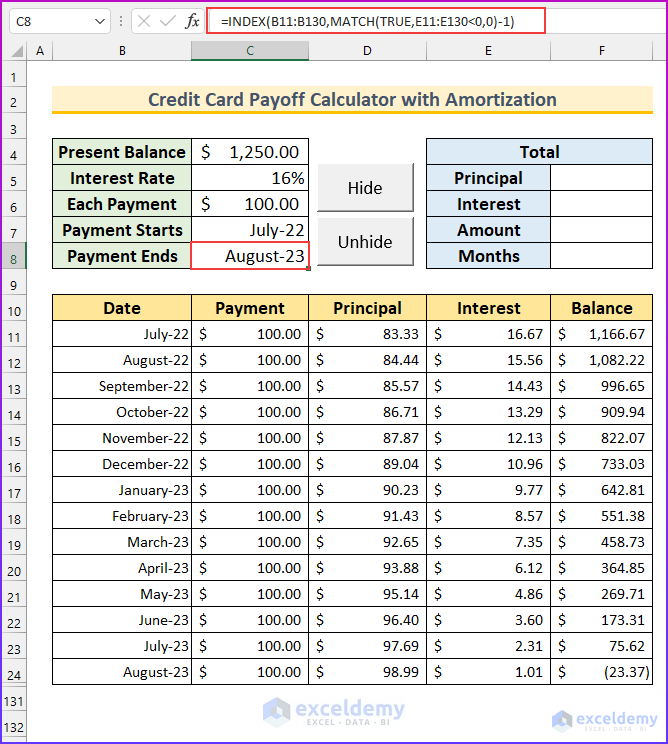
- Firstly, type this formula in cell C8 to find the month when the credit card debt will be paid off.
=INDEX(B11:B130,MATCH(TRUE,E11:E130<0,0)-1)
Formula Breakdown
- MATCH(TRUE,E11:E130<0,0)-1
- Output: 14.
- We find the row number where the interest is negative. Row 15 has a negative interest amount. Then, we subtract 1 from it because we want the row before the first negative number.
- Our formula reduces to INDEX(B11:B130,14)
- Output: 45139.
- This means August, 2023.
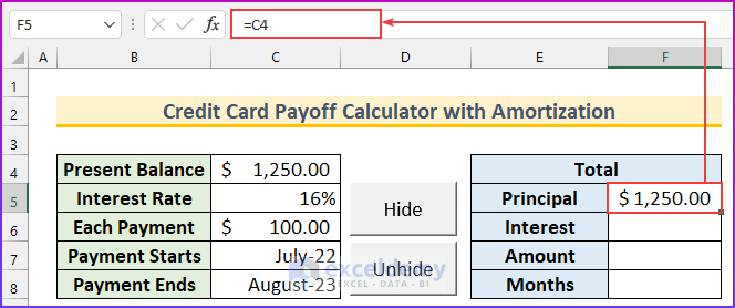
- Then type another formula in cell F5.
=C4
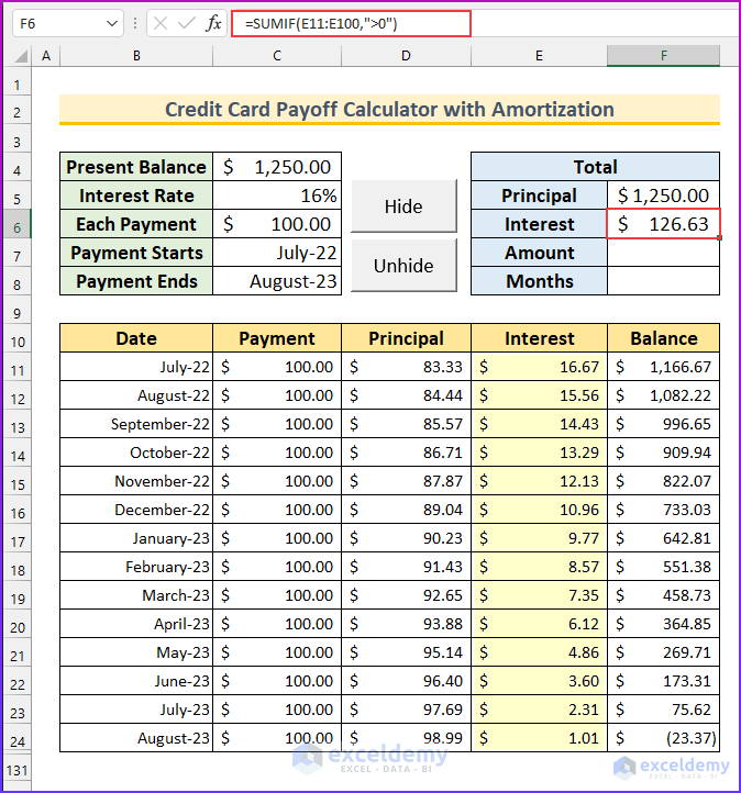
- Afterward, type this formula in cell F6 to find the amount of total interest.
=SUMIF(E11:E100,">0")
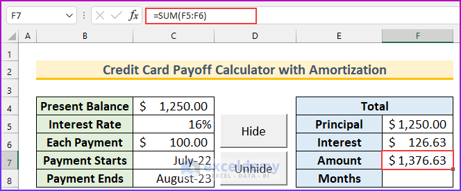
- Then, type this formula in cell F7 to find the total amount paid.
=SUM(F5:F6)
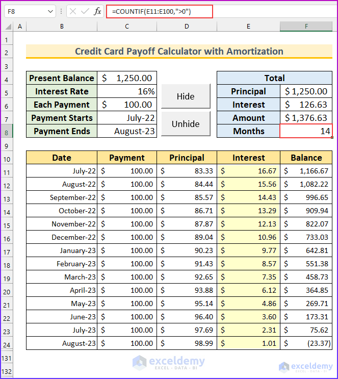
- Lastly, type this formula in cell F8 to find the number of months required to payoff the credit card debt.
=COUNTIF(E11:E100,">0")
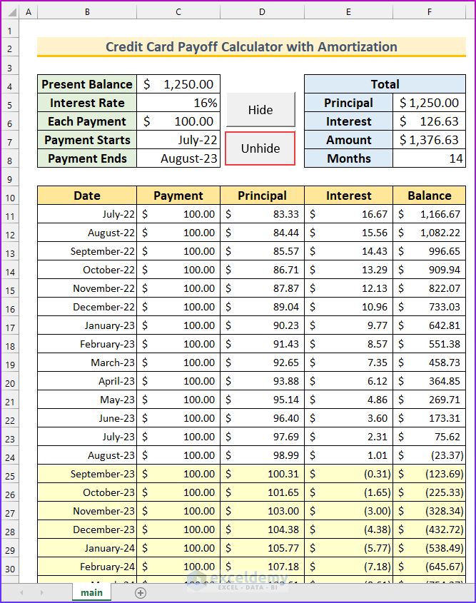
- Now, we can click on the “Unhide” button to show all the hidden rows.
Read More: How to Create a Credit Card Payoff Spreadsheet in Excel
Download Practice Workbook
Conclusion
We have shown you five quick steps to create a credit card payoff calculator with amortization in Excel. If you face any problems regarding these methods or have any feedback for me, feel free to comment below.
Related Articles
- How to Create Credit Card Payoff Calculator with Snowball in Excel
- Create Multiple Credit Card Payoff Calculator in Excel Spreadsheet
<< Go Back to Credit Card Payoff Calculator | Finance Template | Excel Templates
Get FREE Advanced Excel Exercises with Solutions!
