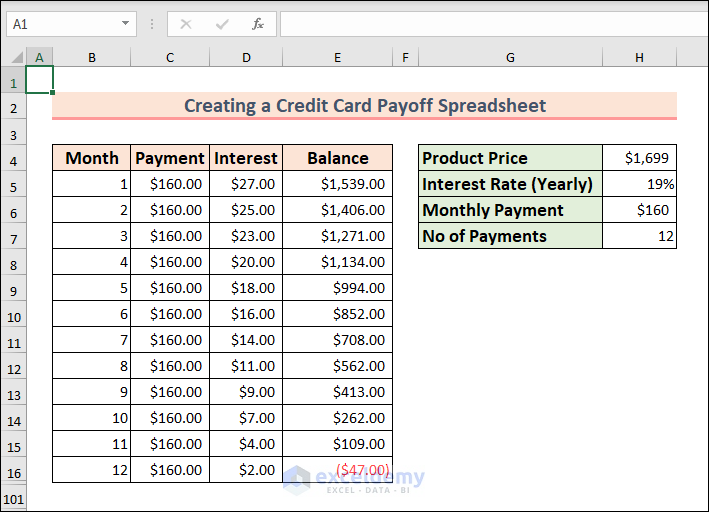
How to Create a Credit Card Payoff Spreadsheet in Excel

This is a quick view of the credit card payoff spreadsheet used in the first method.

Method 1 – Creating a Credit Card Payoff Spreadsheet Manually

Use the NPER function to calculate the number of payments to pay off the debt. Apply the SEQUENCE function to auto-populate the number of months column in the dataset.

Steps:

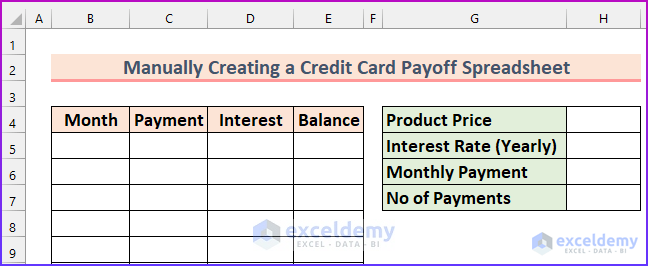
Enter the column headings:
- Month.
- Payment.
- Interest.
- Balance.
Enter the headings for debt information:
- Product Price → The total debt to buy a product.
- Interest Rate (Yearly) → The annual interest rate.
- Monthly Payment → The amount paid per month.
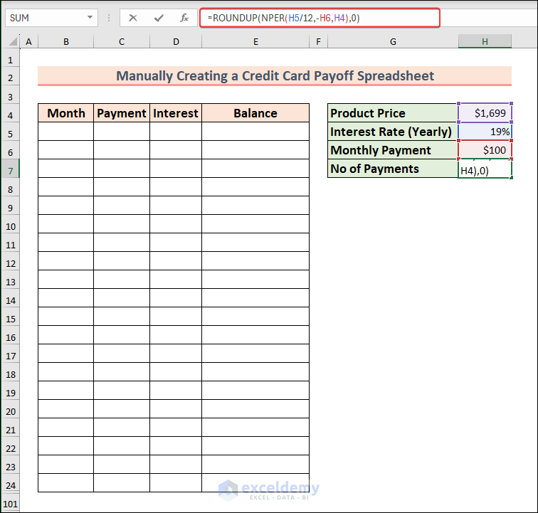
- No of Payments → Find this value using the NPER function.

Enter this formula in H7 and press ENTER.

=ROUNDUP(NPER(H5/12,-H6,H4),0)

Formula Breakdown

The interest rate is divided by 12 to find the monthly interest rate from the yearly interest rate.
A negative sign is used in the monthly payment amount to indicate it as a negative cash flow.
The product price is used as the present value.

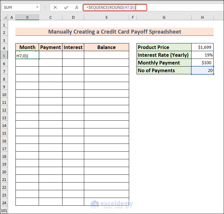
Enter this formula in B5. It will AutoFill the number of months by incrementing them by 1. The ROUND function rounds the number of payments value. You can always use the ROUNDUP function to round up.

=SEQUENCE(ROUND(H7,0))

Press ENTER and enter this formula in C5 (It refers to the monthly payment value). Drag the Fill Handle, to apply the formula to the rest of the cells.

=$H$6

To find the balance (after the first iteration) enter this formula in E5.

=H4-C5

Enter this formula in D5 and drag it down. It will find the interest amount accrued for each month. It divides the value by 12 to use the monthly interest rate value. To calculate the daily interest rate, you will need to divide it by 365.

=ROUND((E5+C5)*$H$5/12,0)

Add the interest amount to find the balance in the rest of the cells.
Enter this formula in E6 and drag down the Fill Handle.

=E5+D5-C6

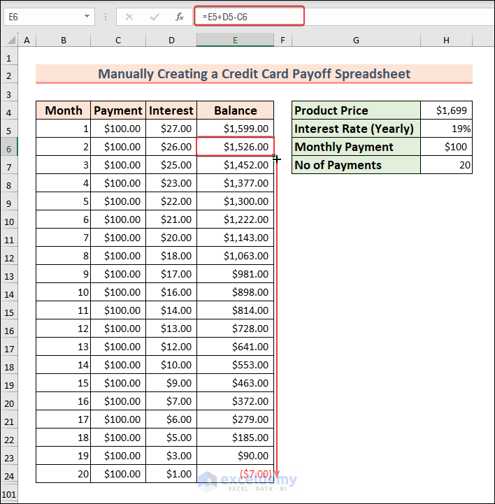
The credit card payoff spreadsheet is created.

If you change any of the values ( 200 as a monthly payment), the spreadsheet will update.
There are extra rows:

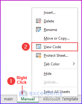
Use a VBA code to hide the rows that have empty values in column B .
Right-click the sheet and select View Code.

Use the following code.

Option Explicit
Private Sub Worksheet_Change(ByVal Cell_Target As Range)

    Dim Cell_Range As Range
    Application.ScreenUpdating = False
        For Each Cell_Range In Range("B7:B100")
            If Cell_Range.Value = "" Then
                Cell_Range.EntireRow.Hidden = True
        
            Else
                Cell_Range.EntireRow.Hidden = False
            End If
        Next Cell_Range
    Application.ScreenUpdating = True
End Sub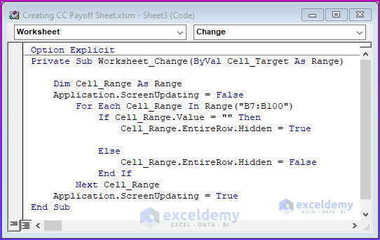

VBA Code Breakdown

A Private Sub procedure is used.
The variable type is declared.
A For Each Next loop goes through B7:B100. The first range value is set to B7.
If any cell value within that range is blank, the code will set the “EntireRow.Hidden” property to true and hide the rows.
This code will update automatically if the parameters of the credit card are changed.

Save the code.

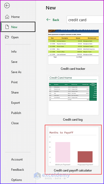
Method 2 – Using a Microsoft Template to Create a Credit Card Payoff Spreadsheet in Excel

Steps:

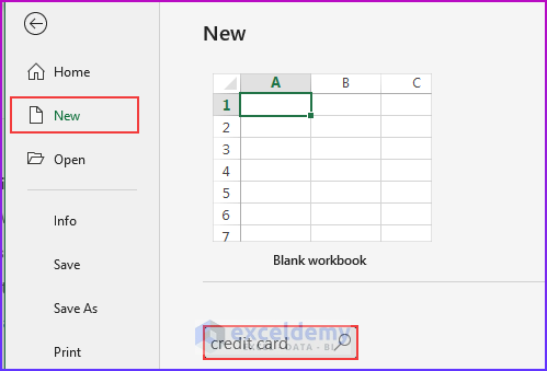
Press ALT, F, N, and the S to activate the search feature and create a new workbook based on a template. Alternatively, go to File → New → enter text in the Search Box.
Enter “Credit Card” and press ENTER.

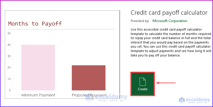
Select “Credit card payoff calculator” .

Click Create.

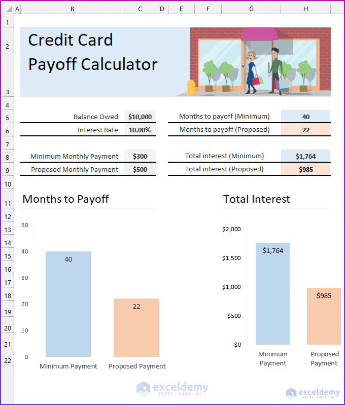
A credit card payoff spreadsheet will be created.
Enter different values and the number of months required to pay off the debt and the total amount of interest will be displayed. There is an option to pay more than the minimum amount.