In this article, we will demonstrate how to create a credit card payoff calculator in Excel using the snowball method.
Debt Snowball Method
When a borrower has more than one debt and repays them by paying off the smallest debts first, we call this technique the “snowball” method. As an example, suppose you have three outstanding debts of $10, $20, and $30, with a minimum payment of $2 in each installment. Using the snowball method, you would pay the total minimum amount of $6, and allocate any additional repayment amounts towards the $10 debt first.
After repaying the the lowest debt, the second-lowest debt will be paid off next, creating a snowball effect. The opposite technique, where the largest debt is repaid first, is called the “avalanche” method.
How to Create a Credit Card Payoff Calculator Using the Snowball Method in Excel
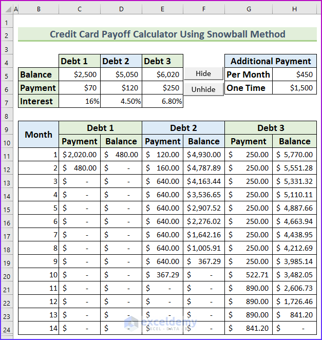
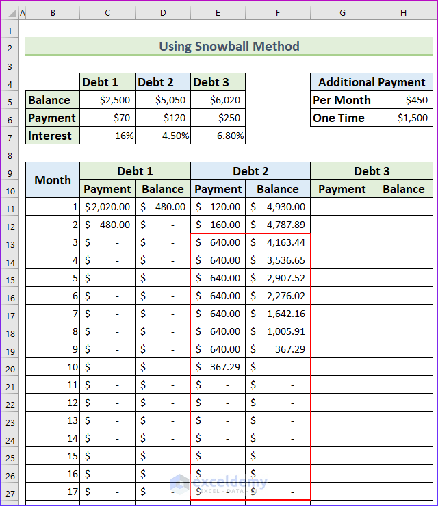
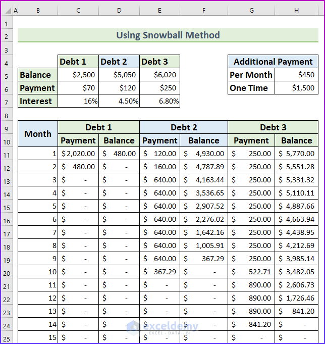
Here is a quick look at the credit card payoff calculator using the snowball method, which we will create in this tutorial.
Step 1 – Setting up the Essentials
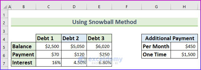
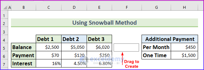
First we’ll input information about the debt, the additional amount to be repaid each month, and a one-time payment. We’ll assume there are 3 debts to be repaid.
- Add a table, containing the following information for each of the 3 debts:
- Balance → The total outstanding debt.
- Payment → The minimum amount that needs to be paid off per month.
- Interest → The annual interest rate.
- Add another table for repayment details with the following information:
- Per Month → The amount we will pay on top of the minimum payment.
- One Time → Any additional one-time payment we might make.
Step 2 – Calculating the First Debt Payoff
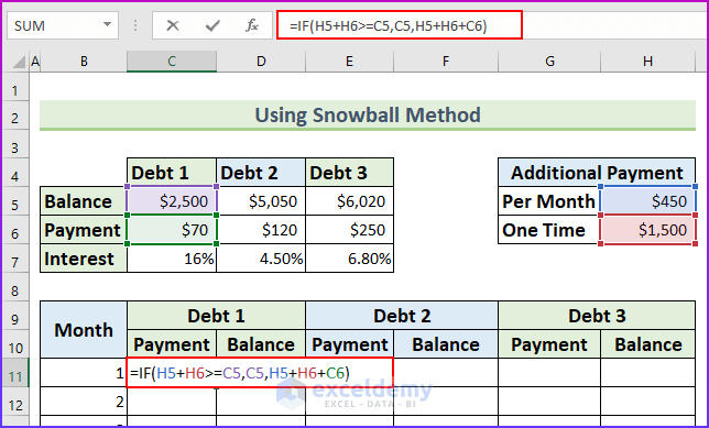
Now we find the repayment amount for the first debt using the IF function.
- Enter the following formula in cell C11:
=IF(H5+H6>=C5,C5,H5+H6+C6)
- Here, if the total amount of the additional payment is more than that of the balance of debt 1, the formula will return the balance from debt 1, else it will add the values of the additional payment and the minimum payment for debt 1.
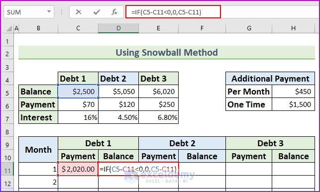
- Enter the following formula in cell D11 to find the balance:
=IF(C5-C11<0,0,C5-C11)
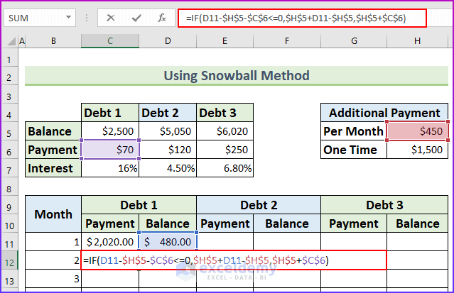
Next, we will create a formula to find the payment values for the second month.
- Enter the following formula in cell C12:
=IF(D11-$H$5-$C$6<=0,$H$5+D11-$H$5,$H$5+$C$6)
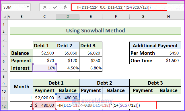
Next, we will find the Balance value for the second month. We divide the yearly interest rate by 12 to find the monthly interest rate.
- Enter the following formula in cell D12:
=IF(D11-C12<=0,0,(D11-C12)*(1+($C$7/12)))
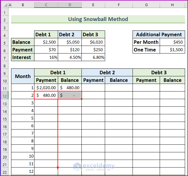
- Drag the cell range C12:D12 down to AutoFill the formula into the cells below .
Read More: How to Create a Credit Card Payoff Spreadsheet in Excel
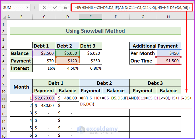
Step 3 – Calculating the Second Debt Payment
Next, we will find the credit card payoff for the second debt.
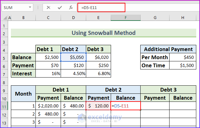
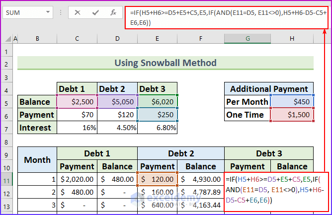
- Enter this formula in cell E11:
=IF(H5+H6>=C5+D5,D5,IF(AND(C11=C5,C11<>0),H5+H6-D5+D6,D6))
- Enter this formula in cell F11:
=D5-E11
- Enter this formula in cell E12:
=IF(AND(((F11-$H$5+C12-D$6-C$6)<=0),D12=0),F11,IF((F11-$D$6-$H$5)<=0,F11,IF(D12=0,$H$5-C12+D$6+C$6,D$6)))
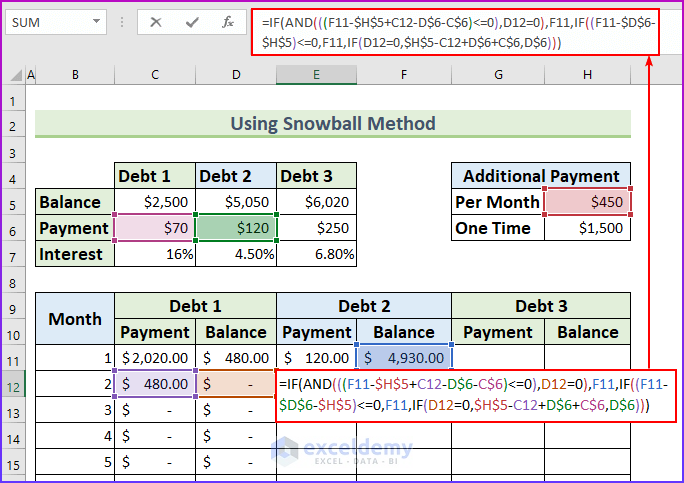
Formula Breakdown
- AND(((F11-$H$5+C12-D$6-C$6)<=0),D12=0)
- Output: False.
- (F11-$D$6-$H$5)<=0
- Output: False.
- IF(D12=0,$H$5-C12+D$6+C$6,D$6)
- Output: 160.
- Reduces to → IF(FALSE,F11,IF((F11-$D$6-$H$5)<=0,F11,160))
- Output: 160.
- Enter this formula in cell F12:
=IF(F11-E12<0,0,(F11-E12)*(1+($D$7/12)))
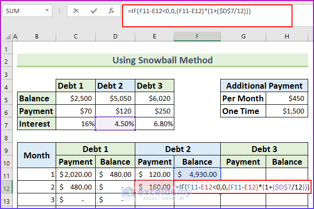
- AutoFill the formulas from the range E12:F12 to the cells below to return the values for debt 2.
Step 4 – Finding the Third Debt Payment
Now we find the credit card payoff for the last debt using the snowball method.
- Enter this formula in cell G11:
=IF(H5+H6>=D5+E5+C5,E5,IF(AND(E11=D5, E11<>0),H5+H6-D5-C5+E6,E6))
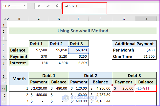
- Enter this formula in cell H11 to find the first balance:
=E5-G11
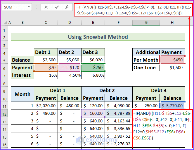
- Enter this formula in cell G12:
=IF(AND(((H11-$H$5+E12-E$6-D$6-C$6)<=0),F12=0),H11, IF((H11-$E$6-$H$5)<=0,H11,IF(F12=0,$H$5-E12+E$6+D$6+C$6,E$6)))
Formula Breakdown
- AND(((H11-$H$5+E12-E$6-D$6-C$6)<=0),F12=0)
- Output: False.
- (H11-$E$6-$H$5)<=0
- Output: False.
- IF(F12=0,$H$5-E12+E$6+D$6+C$6,E$6)
- Output: 250.
- Reduces to → IF(FALSE,H11, IF(FALSE,H11,250))
- Output: 250.
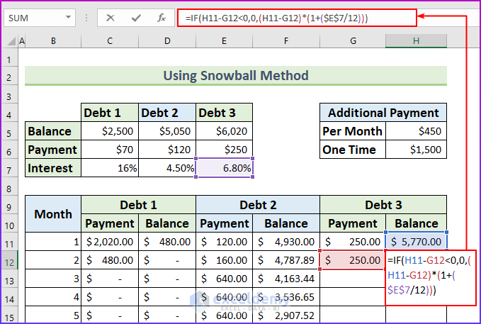
- Enter this formula in cell H12:
=IF(H11-G12<0,0,(H11-G12)*(1+($E$7/12)))
- AutoFill the formula from the cell range G12:H12 to the cells below.
- Fill the formulas down to month 120 (10 years).
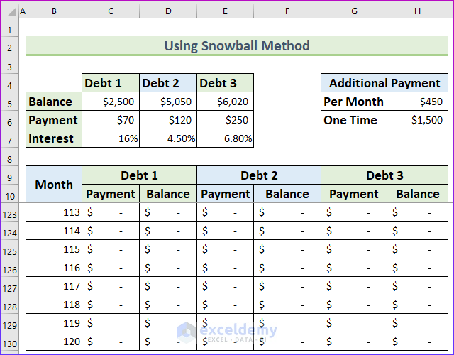
Step 5 – Applying VBA to Hide Extra Rows
We can easily hide the extra rows using Excel VBA macros. After that, we will use another VBA code to unhide the rows.
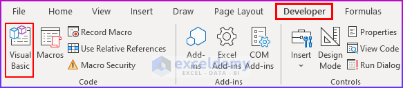
- From the Developer tab → select Visual Basic (or press ALT+F11).
- Click Insert, then select Module.
- Enter the following code in the Module window that opens:
Option Explicit
Sub Hide_Rows()
    Dim Cell_Range As Range
    Application.ScreenUpdating = False
        For Each Cell_Range In Range("G11:G130")
            If Cell_Range.Value = 0 Then
                Cell_Range.EntireRow.Hidden = True
            Else
                Cell_Range.EntireRow.Hidden = False
            End If
        Next Cell_Range
    Application.ScreenUpdating = True
End Sub
Sub Unhide_Rows()
    Rows.EntireRow.Hidden = False
End Sub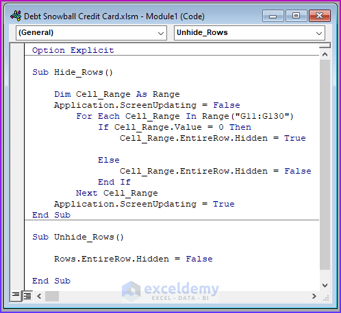
VBA Code Breakdown
- We have two Sub procedures in this VBA code. The first one hides the rows that have 0 in the range G11:G130. We use a For Each Next loop to iterate through all the cell ranges.
- The last Sub simply unhides all the rows in the active sheet.
- Save and Close the Module.
Now we’ll insert two buttons to execute the macros.
- From the Developer tab → Insert → select Button (under Form Controls).
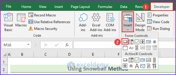
- Drag the cursor to create a box.
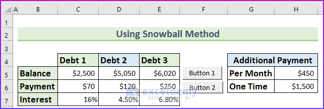
- Repeat this process to create a second box.
We have two buttons in the dataset.
Now, we will assign macros to the buttons.
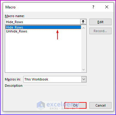
- Right-click on “Button 1” and select Assign Macro.
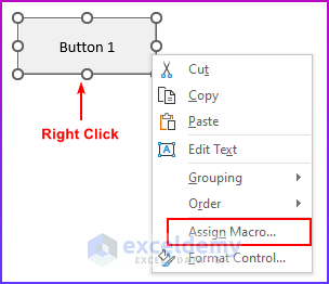
- Select Hide_Rows and click OK.
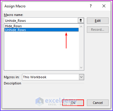
- For the second button, select Unhide_Rows and click OK.
- Change the button labels to Hide and Unhide respectively.
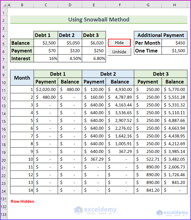
Now, if we press the Hide button, the extra rows will be hidden.
Click on the Unhide button to unhide the rows.
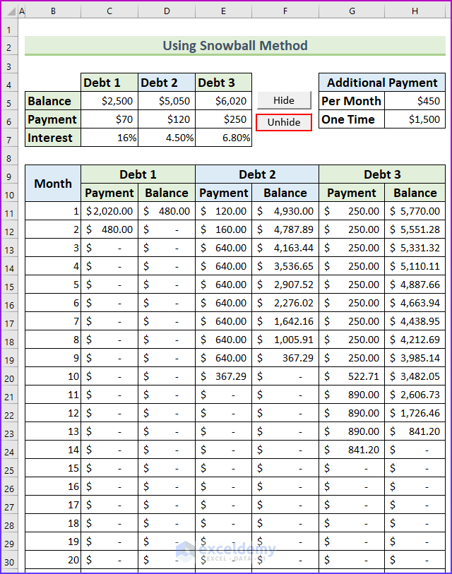
Our snowball credit card payoff calculator is complete.
Download Practice Workbook
Related Articles
- Create Multiple Credit Card Payoff Calculator in Excel Spreadsheet
- Make Credit Card Payoff Calculator with Amortization in Excel
<< Go Back to Credit Card Payoff Calculator | Finance Template | Excel Templates
Get FREE Advanced Excel Exercises with Solutions!
