Credit Card Payoff Calculator in Excel (Create & Use)

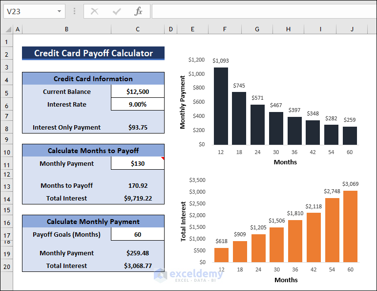
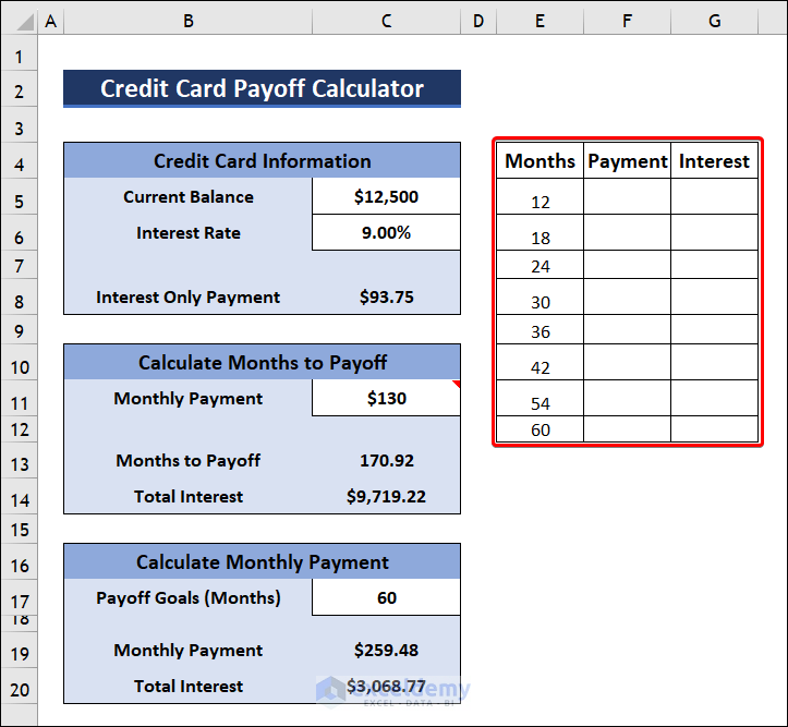
Let’s build this credit card payment calculator so you can determine how much a credit card is costing you. Here’s an overview of what the final result looks like.

Download the Practice Workbook

Download this credit card payoff calculator template you can use to follow along or input your values.

How to Create a Credit Card Payoff Calculator in Excel

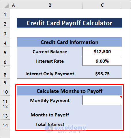
Step 1 – Insert Credit Card Information

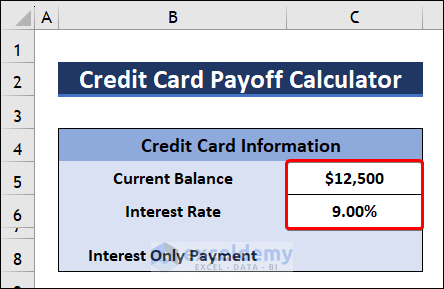
• Create a table named Credit Card Information.

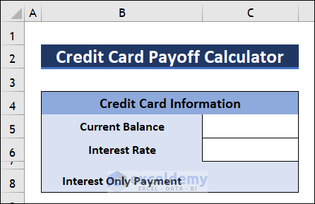
• Insert the Current Balance and Interest Rate of the card.

• Select cell C8 and insert the following formula to calculate Interest Only Payment.

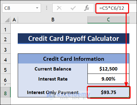
Step 2 – Calculate Months to Payoff

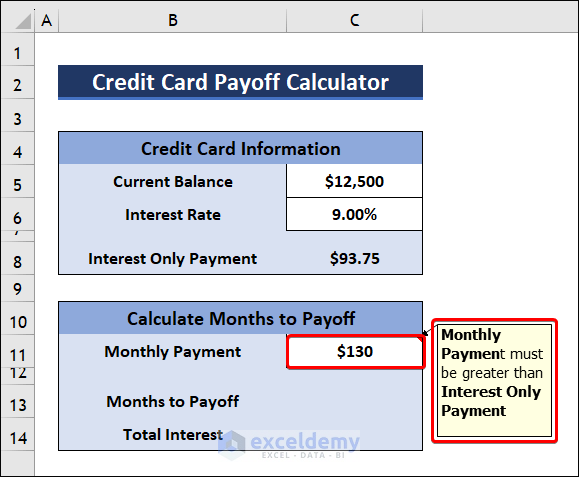
• Insert a table to calculate Months to Payoff.

• Enter the Monthly Payment amount which must be higher than Interest Only Payment. Don’t forget to add a note for the users.

• Use the formula given below to determine Months to Payoff.

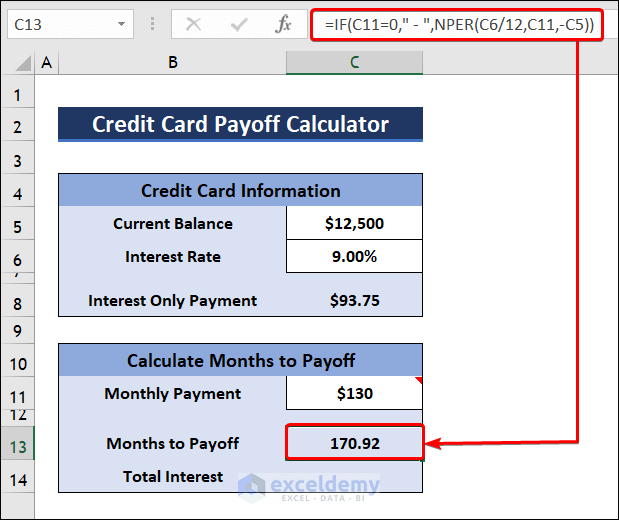
• To calculate Total Interest, insert the following formula:

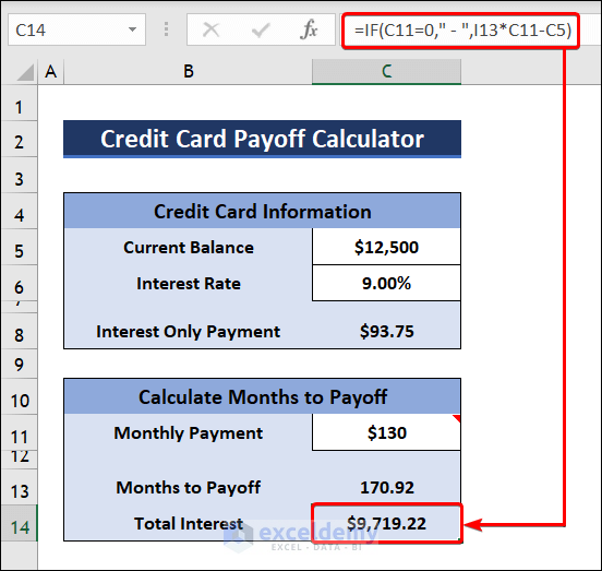
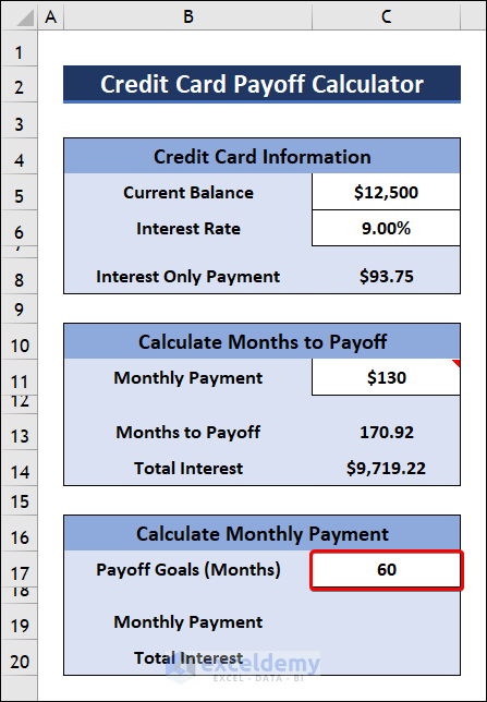
Step 3 – Calculate Monthly Payments

• Create a table to determine Monthly Payment.

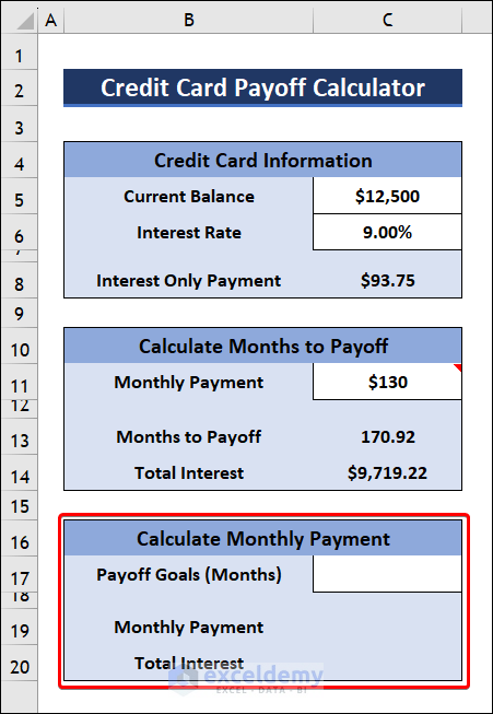
• Write Payoff Goals value in months in cell C17.

• Click on cell C19 and apply the formula below to find the Monthly Payment.

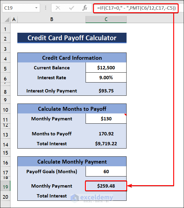
• Copy the following formula in cell C20 to calculate the Total Interest.

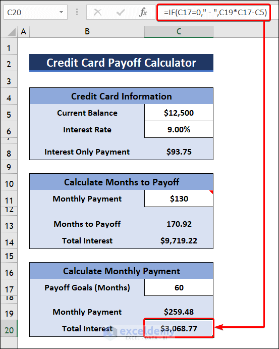
Step 4 – Create and Format a Chart

• Create an additional table to insert charts.
• This table contains Months, Payment, and Interest columns.

• Enter the following formula in the Payment column to determine payments after the corresponding months.

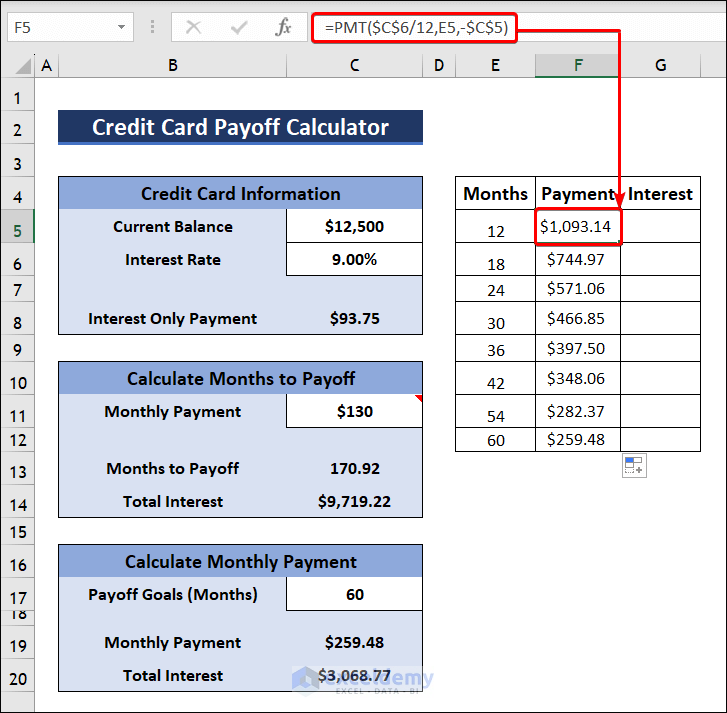
• To calculate Interest, use this formula:

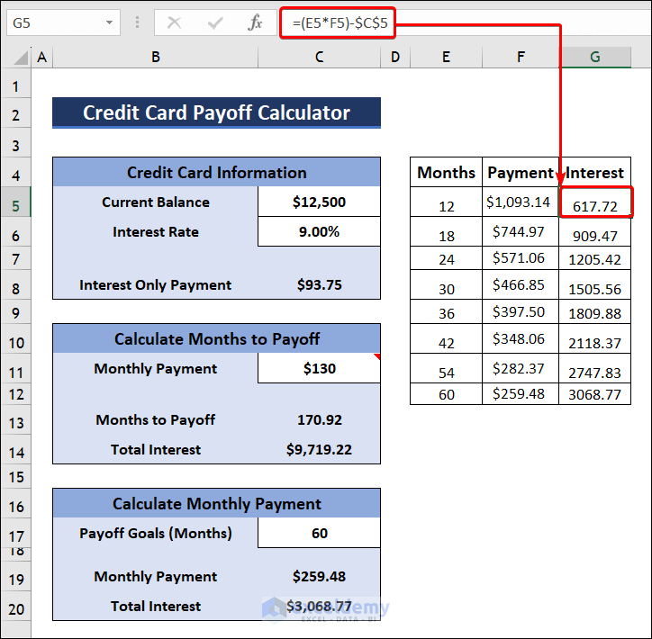
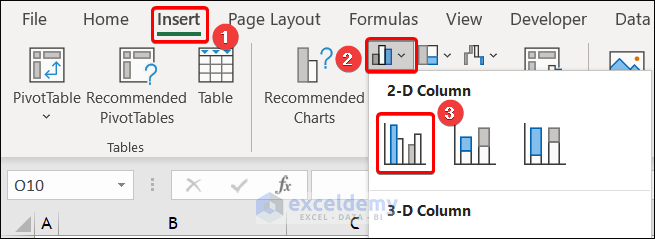
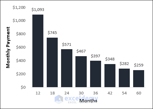
• Go to the Insert tab and select 2-D Column to insert a column chart.

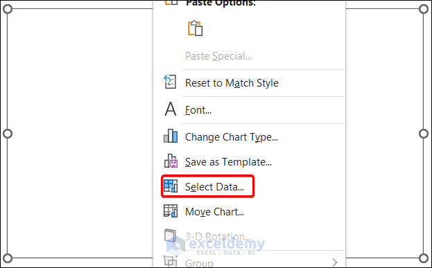
• Right-click on the chart and choose Select Data.

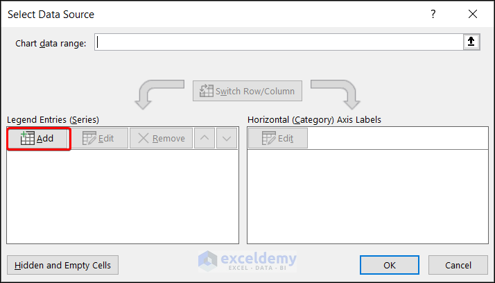
• Click on Add to add a new series.

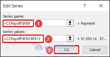
• Write any Series name you want and insert Series values as F5:F12.

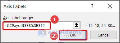
• Click on Edit under Horizontal (Category) Axis Labels.

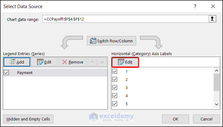
• Use E5:E12 as Axis label range.

• You can format your chart.

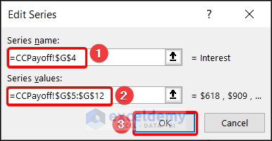
• Add another series and insert a Series name.
• Enter the G5:G12 range as Series values and click the OK button.

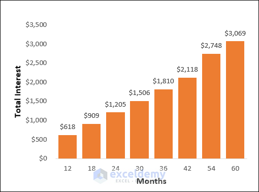
• The Total Interest vs. Months chart will be created.

• The Excel credit card payoff calculator will look like the following image.

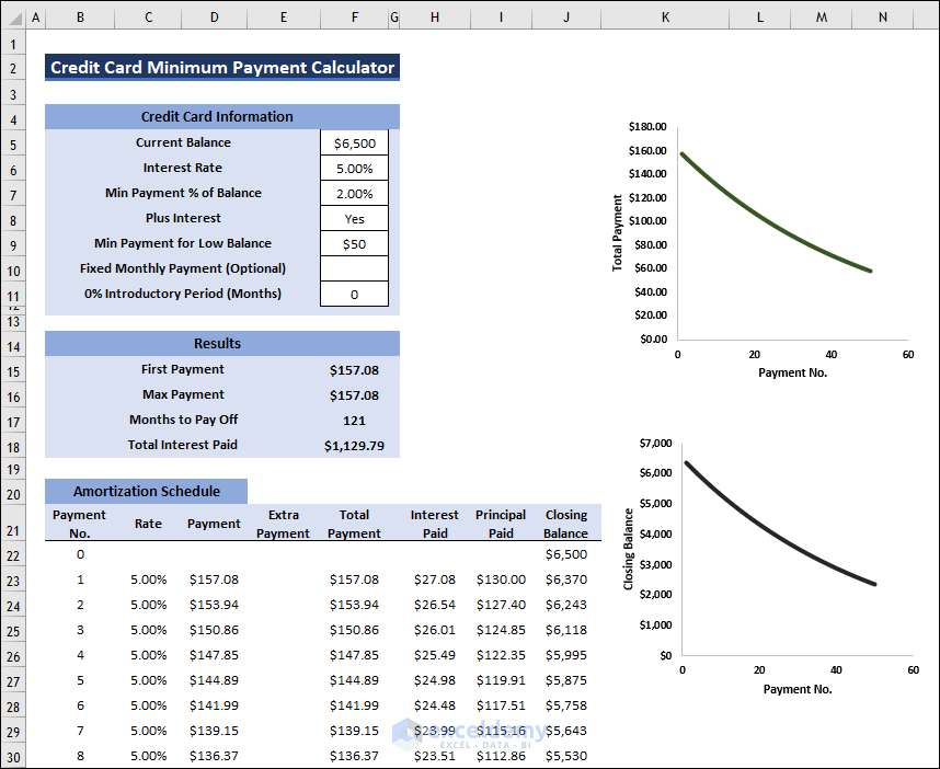
How to Create a Credit Card Minimum Payment Calculator in Excel

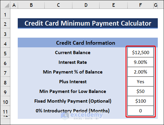
Step 1 – Insert Credit Card Information

• Create a table to insert the necessary credit card information.

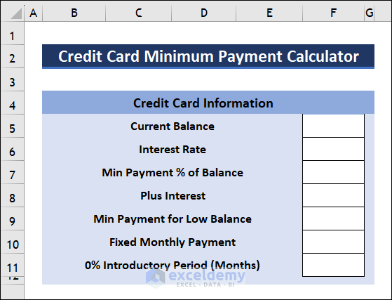
• Enter Current Balance, Interest Rate, Min Payment % of Balance, etc. as inputs.

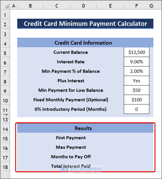
• Insert another table to determine the results.

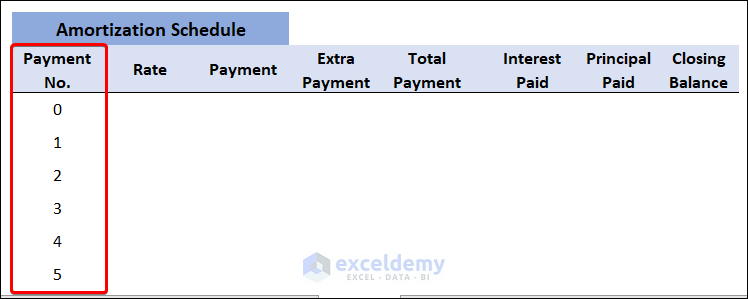
Step 2 – Create an Amortization Schedule

• Create an Amortization Schedule.
• Name the first column Payment No. and insert payment numbers.

• In the second column, copy the following formula to calculate the Rate:

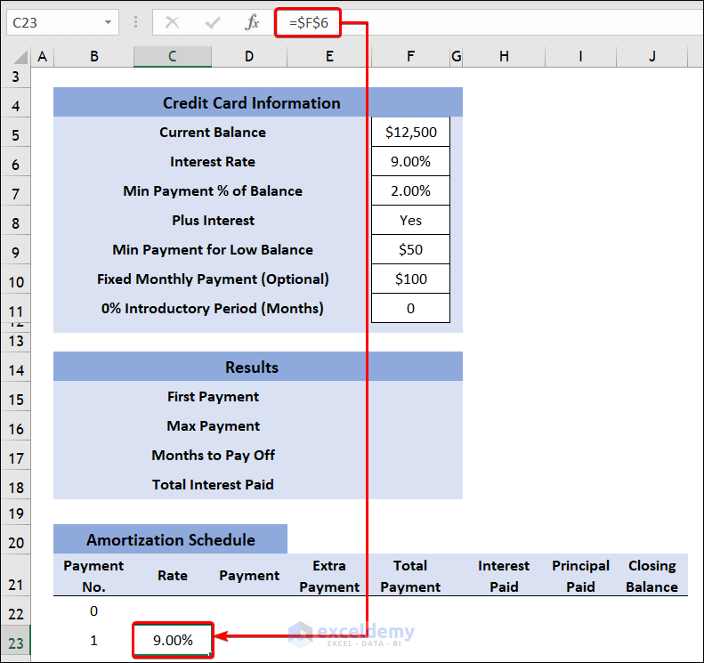
• Apply this formula in the first row to calculate the initial Closing Balance.

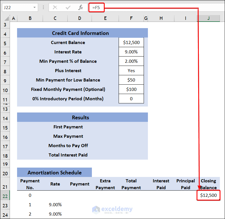
• Select cell H23 and insert the following formula to calculate the Interest Paid.

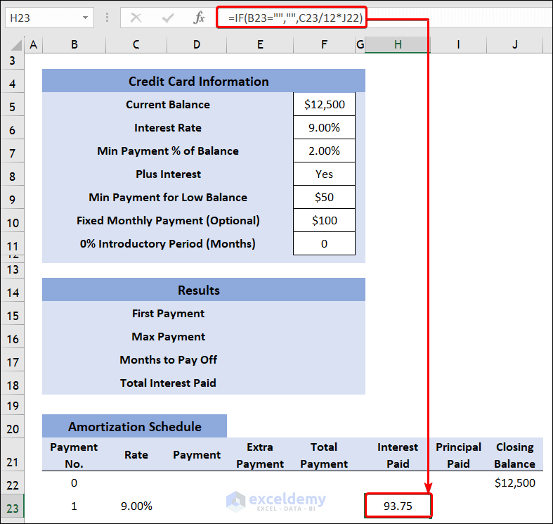
• To calculate Payment, apply this formula in cell D23.

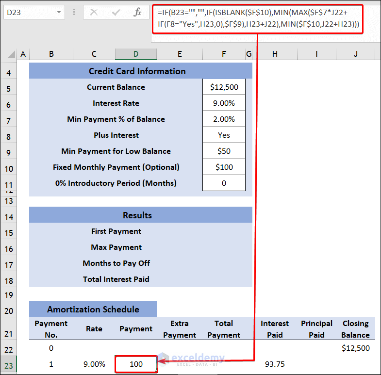
• Use the following formula to find the Total Payment.

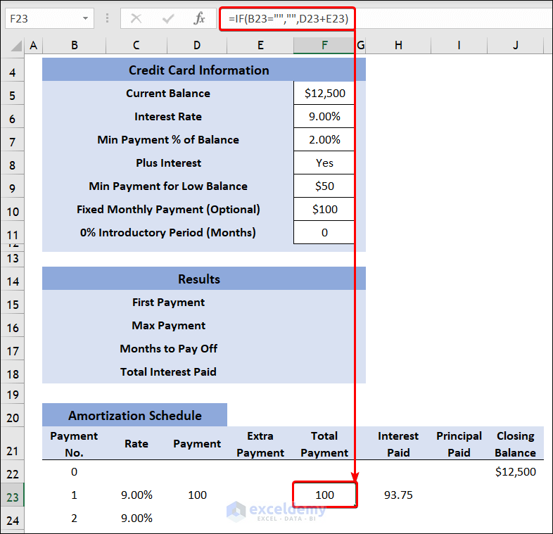
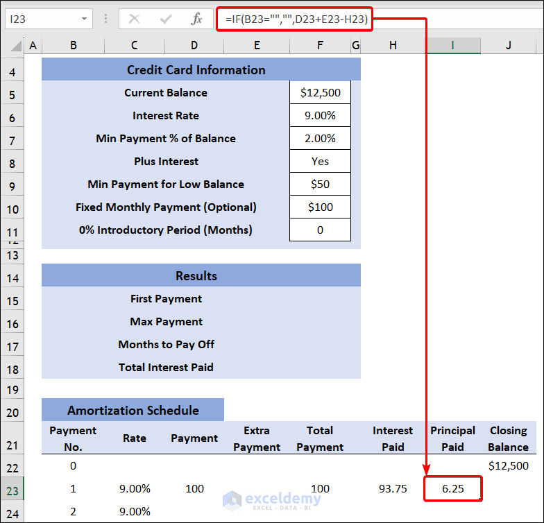
• Select cell I23 and enter the following formula:

• You will get the value of Principal paid.

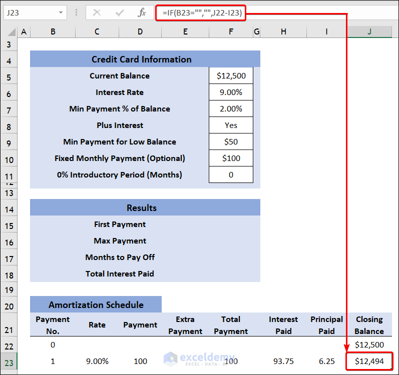
• Apply the following formula to determine the Closing Balance after the 1st payment.

• AutoFill each column of the Amortization Schedule.

Step 3 – Calculate Results

• Insert the following formula in cell F15 to get the value of First Payment.

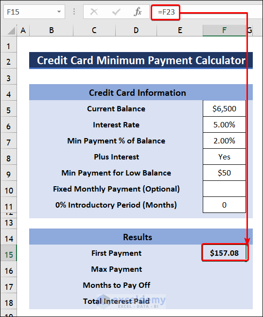
• Calculate Max Payment by using the formula given below:

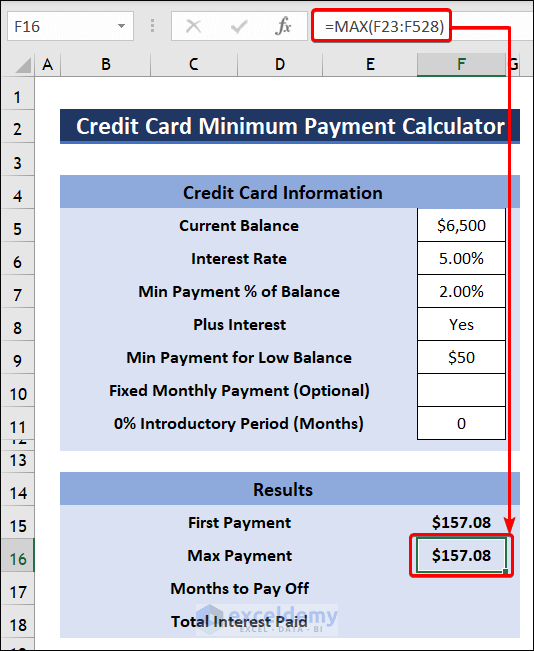
• Insert this formula in cell F17 to find the value of Months to Payoff:

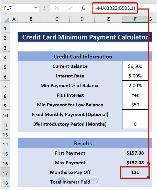
• Enter the following formula and determine Total Interest Paid:

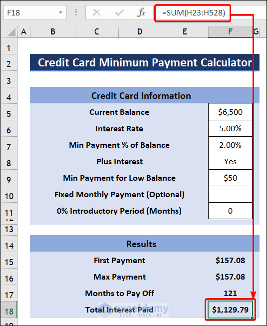
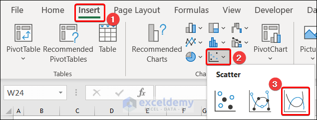
Step 4 – Insert and Format Charts

• Go to Insert and select Scatter or Bubble Chart.]
• Choose Scatter with Smooth Lines.

• Right-click on the chart and choose Select Data.

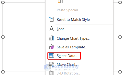
• Click on Add.

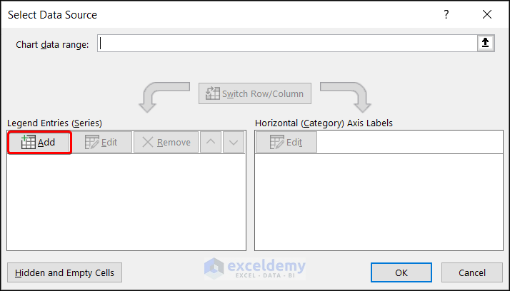
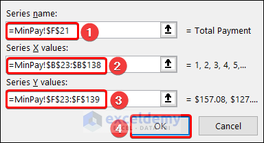
• Write or choose a Series name.
• Use B23:B138 as Series X values and F23:F139 as Series Y values and click on the OK button.

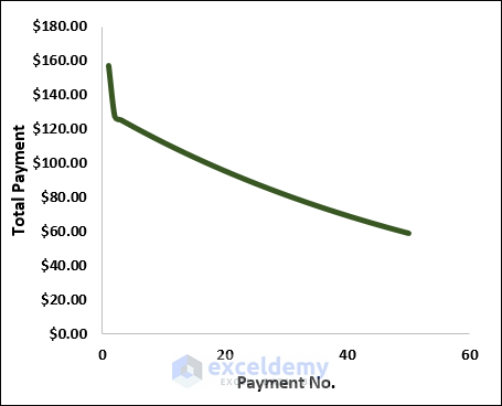
• The Total Payment vs. Payment No. chart will be created.

• Create a Closing Balance vs. Payment No. in a similar way.

• You will get the finalized Credit Card Minimum Payment Calculator.

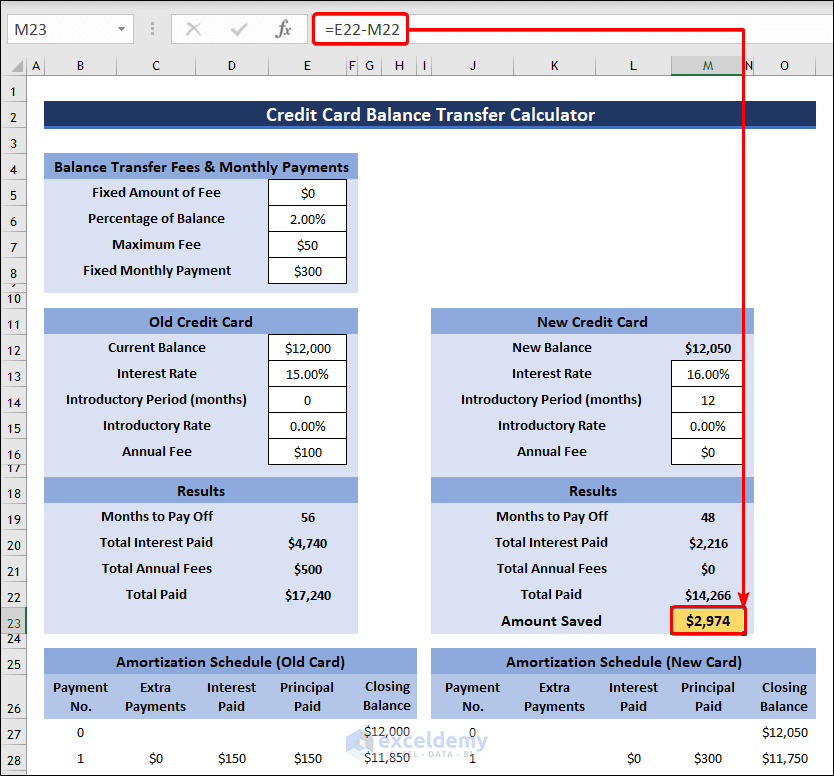
How to Make a Credit Card Balance Transfer Calculator in Excel

Step 1 – Enter Credit Card Information

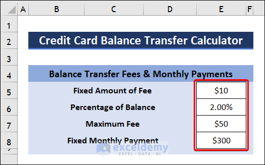
• Create a table to insert all the necessary inputs.

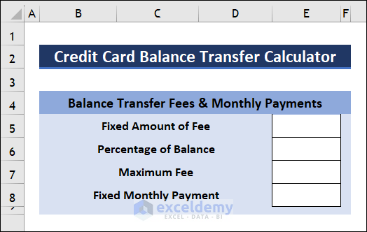
• Enter the values in cells E5 to E8 which are required for calculations.

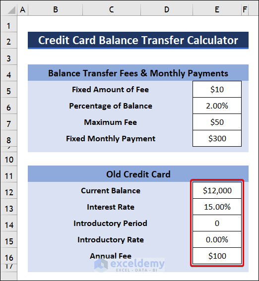
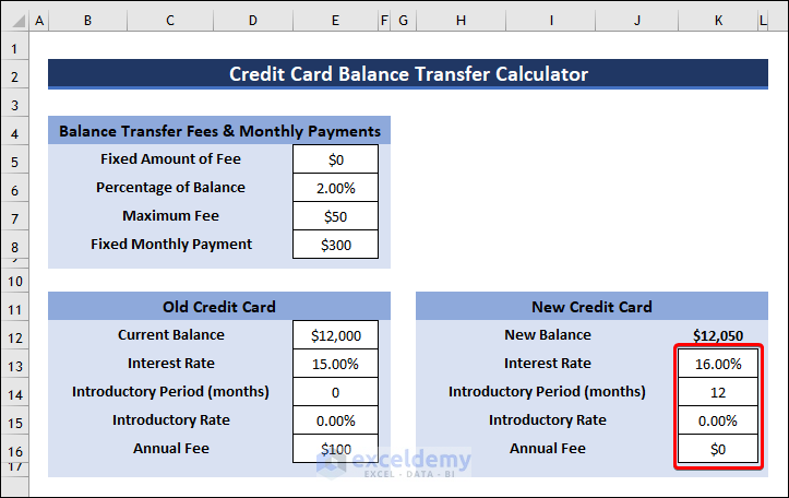
• Enter your Old Credit Card information in a new table.

• Create another table for the New Credit Card.
• Apply the following formula in cell K12 to calculate the New Balance of the new card.

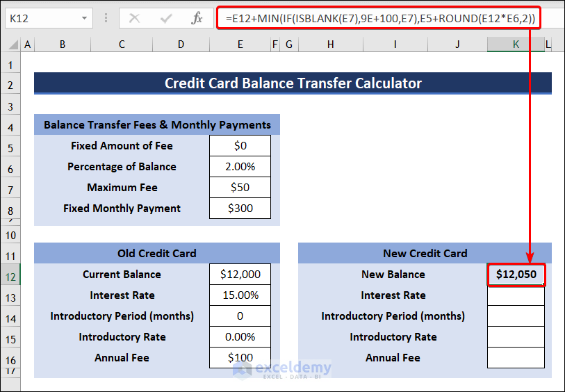
• Insert all the necessary information of the new card in cells K13 to K16.

Step 2 – Create an Amortization Schedule

• Create two Amortization Schedules: one for the old card and the other for the new card.
• Apply the formula below to calculate the initial Closing Balance.

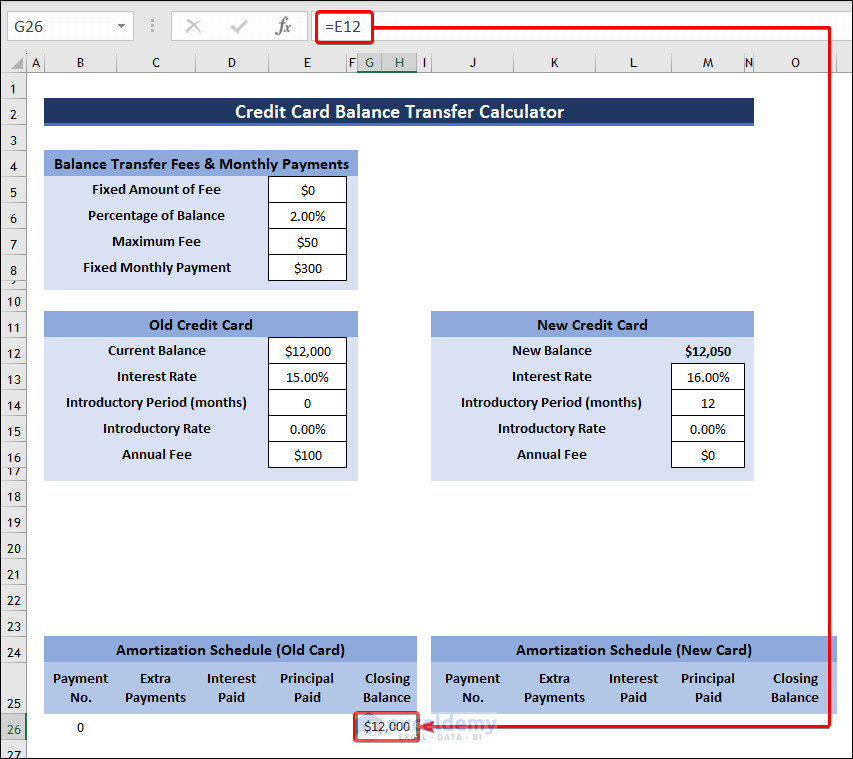
• Enter 0 in the first row of Payment No. column.
• Select cell B27 and use this formula to determine Payment No.

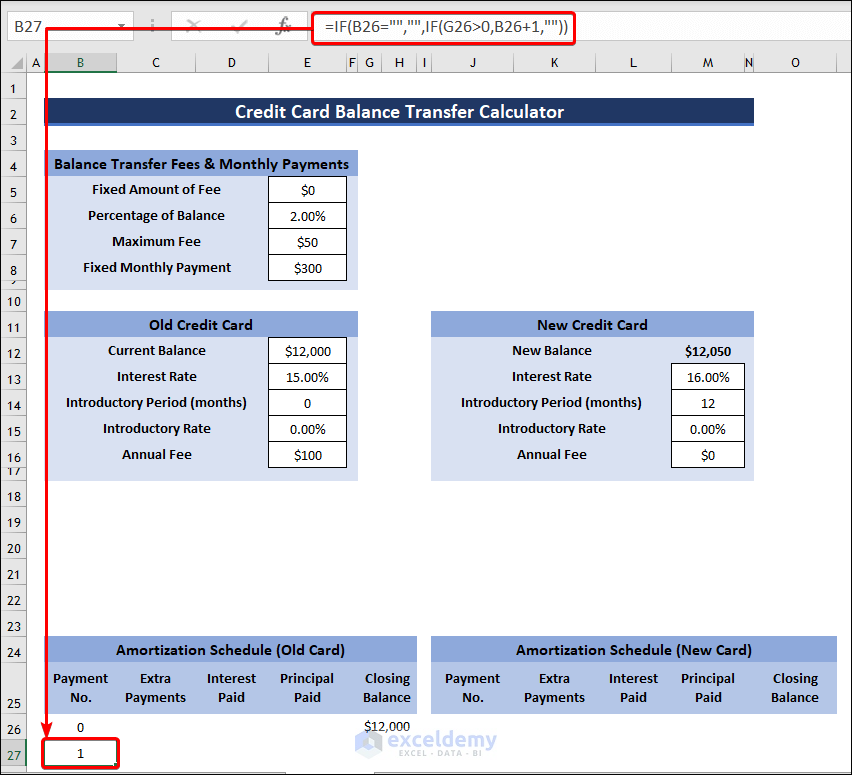
• Calculate Interest Paid by using the following formula.

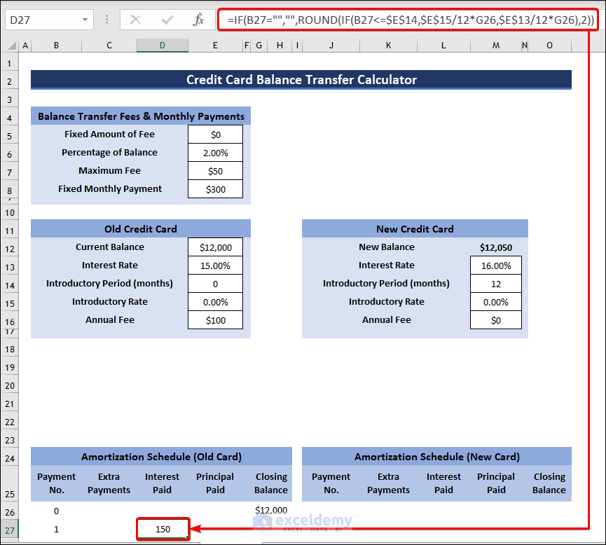
• Use the formula given below to determine Principal Paid.

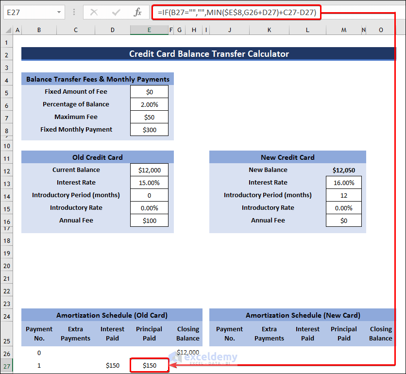
• Click on cell G27 and enter this formula to find the Closing Balance after 1st payment.

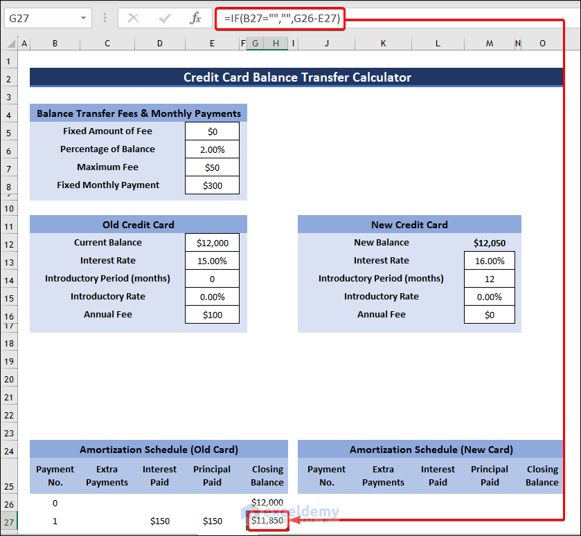
• Determine the initial Closing Balance of the new card with the following formula:

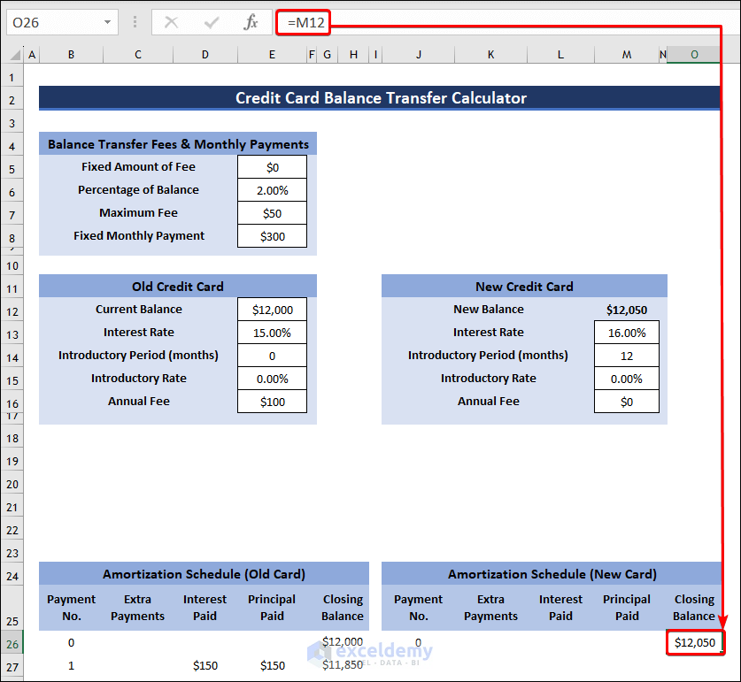
• Calculate Payment No. with the following formula:

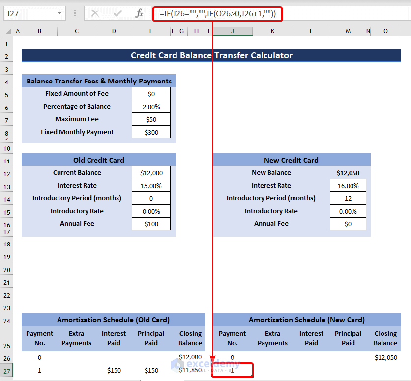
• Determine Interest Paid by applying this formula:

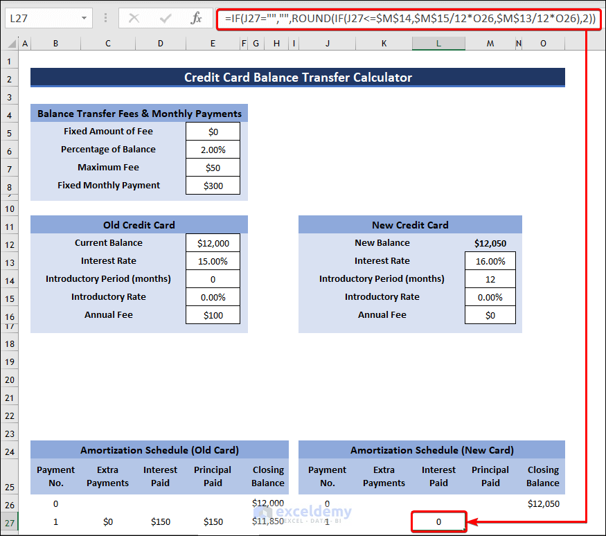
• Insert the formula given below to find Principal Paid:

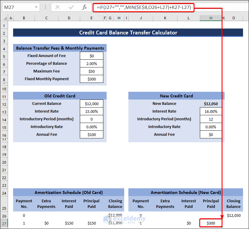
• Determine the Closing Balance after 1st payment with the following:

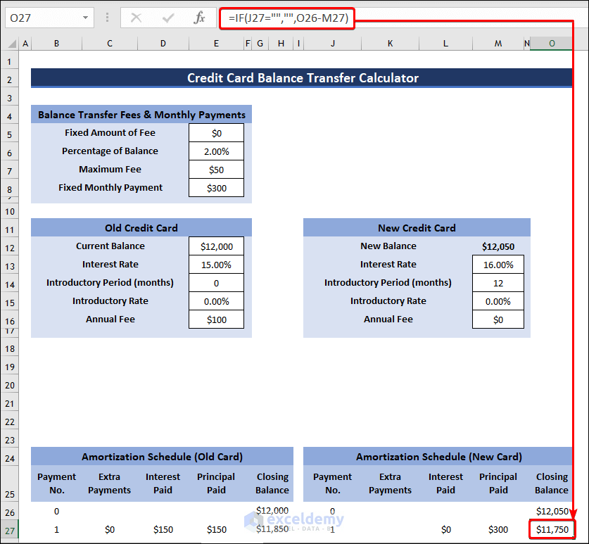
Step 3 – Find the Results

• Select cell E19 and insert the formula given below.

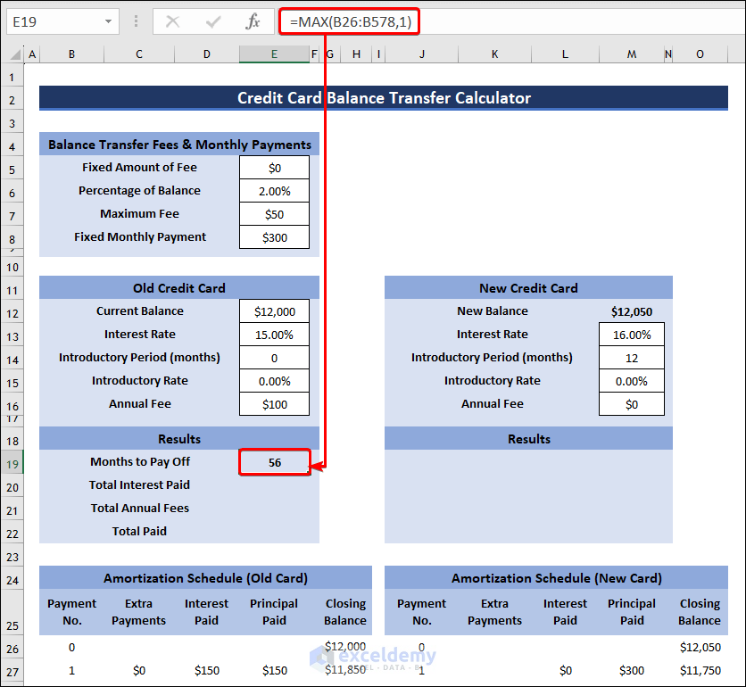
• Sum up all the interest paid amount to calculate the Total Interest Paid:

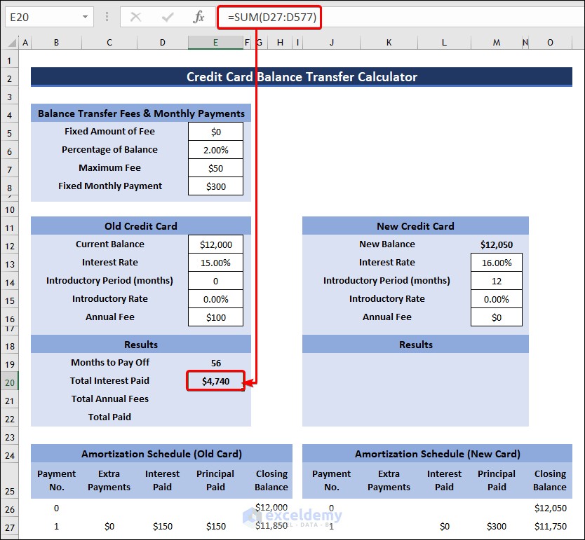
• Insert the following formula and find Total Annual Fees:

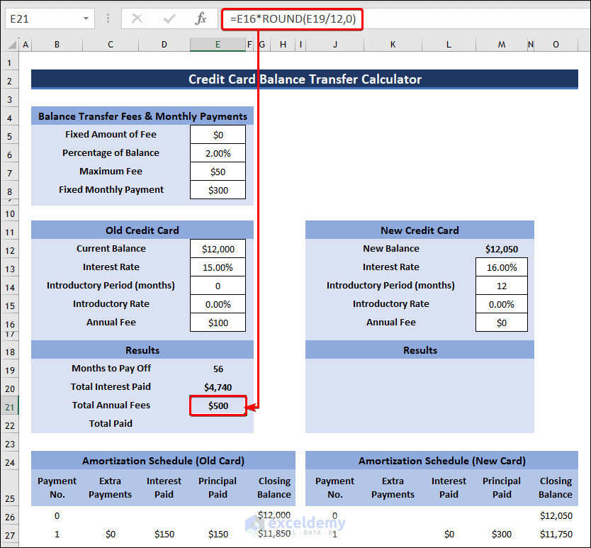
• Determine the Total Paid amount by applying this formula:

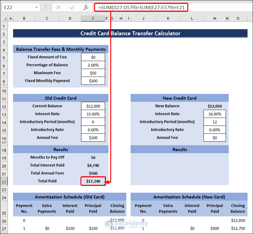
• Calculate Months to Payoff of the new card with the formula given below:

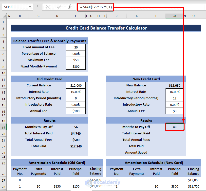
• Add up all the interest paid from the amortization schedule using this formula:

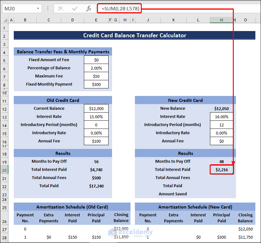
• Determine Total Annual Fees by applying the following formula:

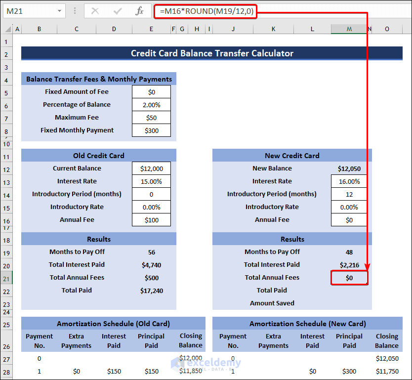
• You can calculate the Total Paid amount using the formula given below:

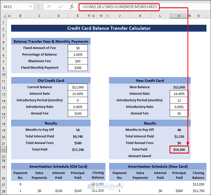
• Select cell M23 and insert the formula given below.

• Press Enter to find the Amount Saved.

Step 4 – Create and Format Charts

• Insert a Scatter with Smooth Lines chart and add a new data series as shown in the previous methods.
• In the Edit Series box, insert range B27:B327 as Series X values and range G27:G327 as Series Y values for old credit card.

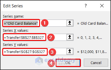
• Similarly, insert range J27:J327 as Series X values and range O27:O327 as Series Y values for the new credit card.

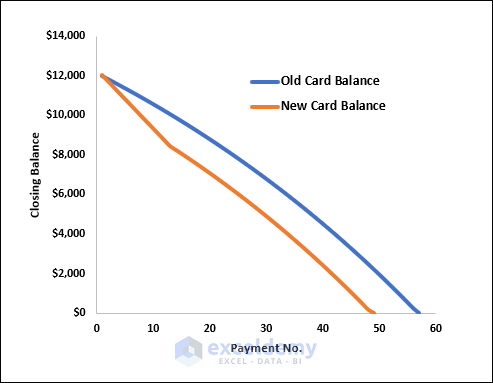
• You will get a chart with old and new credit card balances.

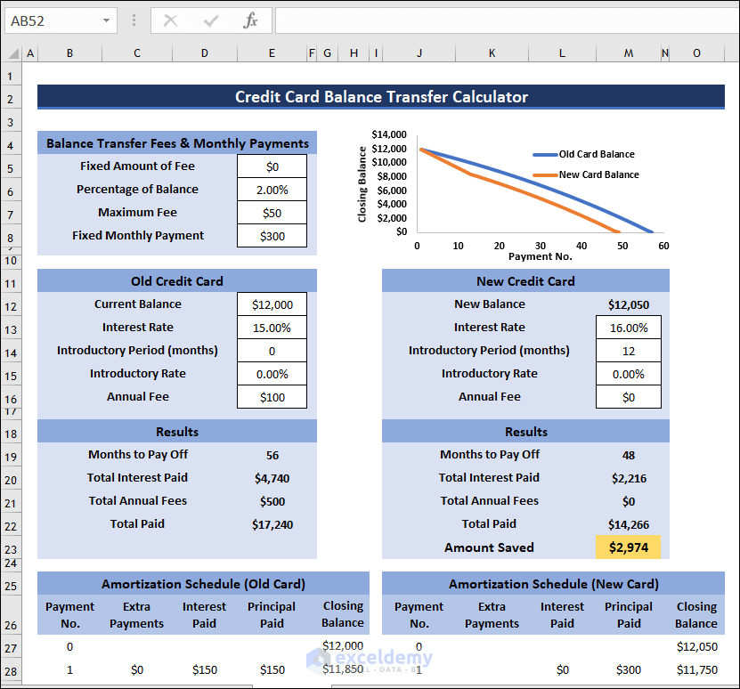
• The overview of the calculator will look like the following image.

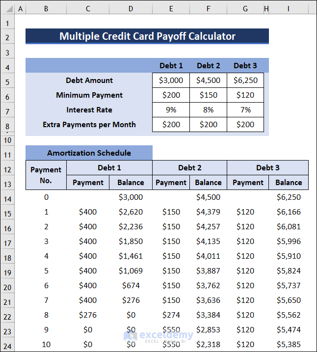
How to Create a Multiple Credit Card Payoff Calculator (Snowball) in Excel

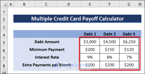
• Create a table and arrange your debts from smallest to largest.
• Enter other necessary information as shown in the image.

• Create an Amortization table and insert the initial Closing Balances of all three debts in the first row.
• Select cell B15 and use the below formula to determine Payment No.

• Apply this formula in cell C15 and find Payment value of Debt 1.

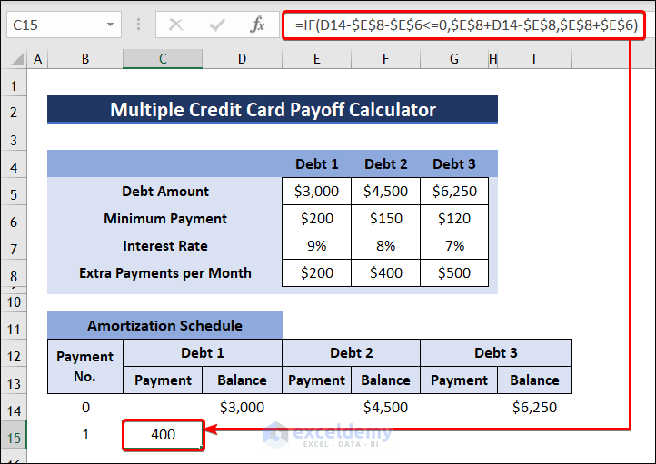
• Insert the following formula to determine the Closing Balance of Debt1 after the first payment.

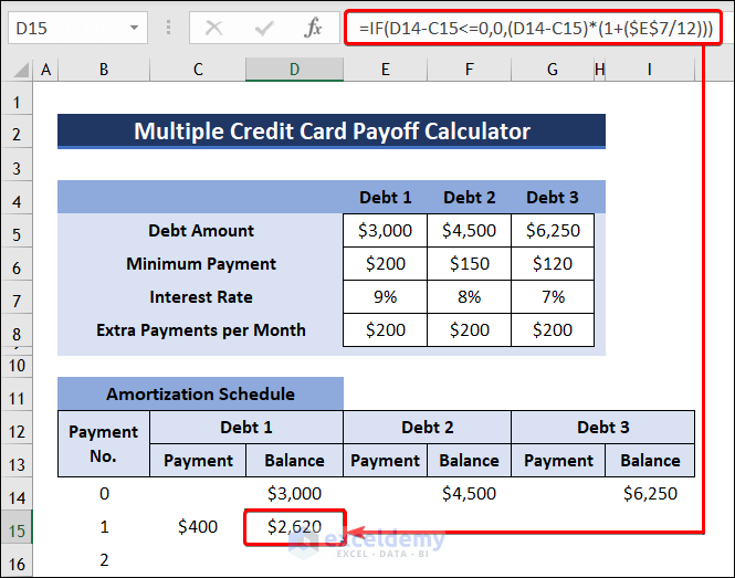
• To calculate Payment of Debt 2, use this formula:

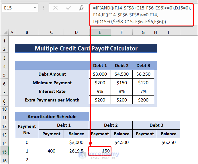
• Click on cell F15 and insert the following formula to get the Closing Balance of Debt 2.

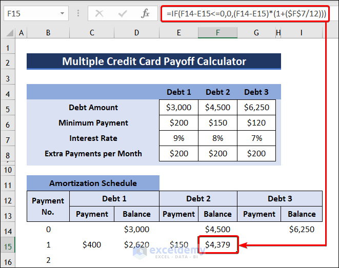
• Apply this formula to find the Payment of Debt 3.

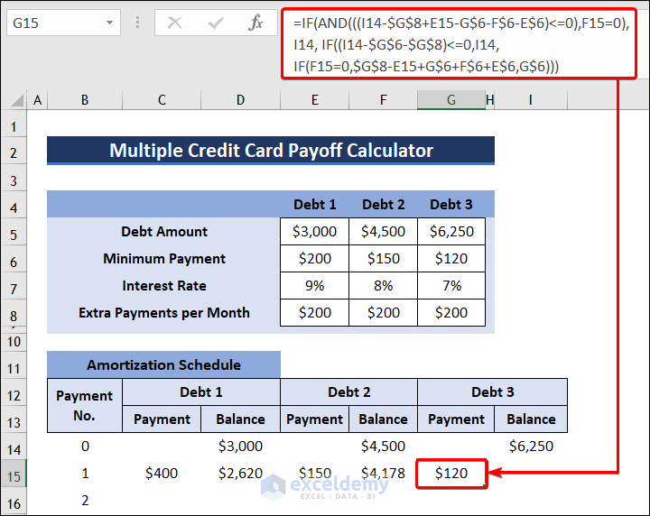
• Calculate the Closing Balance of Debt 3 with the following formula:

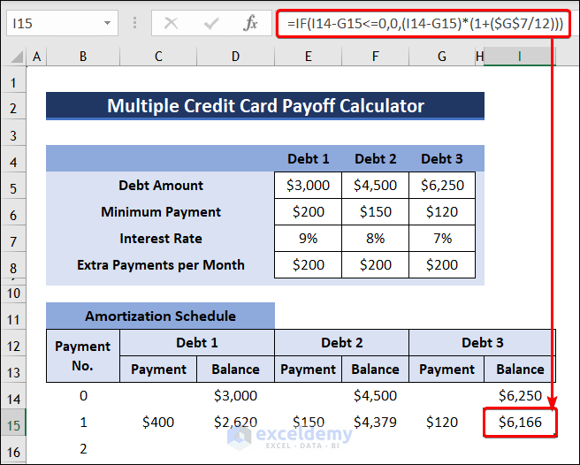
• You can insert a chart to show the Closing Balance against Payment No. following the steps discussed above.

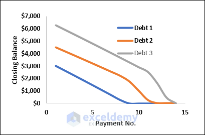
• The calculator will look like the following image.

Things to Remember

• The Monthly Payment must be larger than Interest Only Payment.
• Make sure to arrange the debts from smallest to largest while using the snowball method.

Frequently Asked Questions

1. What is the total payoff?

The total payoff is the amount you have to pay to completely payoff your debt or loan. The payoff amount is not the same as the current amount. The payoff amount might include interest as well as other fees. Therefore, the payoff amount is more than what you owe.

2. How do you calculate percentage of debt paid?

Add up all your debts and rent. Then divide the total by your monthly income. Multiply it by 100% to convert the ratio into percentage.

3. How do I pay off my multiple debts using Excel?

You can use the snowball method to pay off your multiple debts. In this method, you will have pay off your smallest debt first. Once this debt is paid, you use this money to pay off your next smallest debt. You can use the Multiple Credit Card Payoff Calculator given above in this article for this purpose.

Credit Card Payoff Calculator Excel: Knowledge Hub

• Create a Credit Card Payoff Spreadsheet
• Credit Card Payoff Calculator with Amortization
• Create Multiple Credit Card Payoff Calculator
• Create Credit Card Payoff Calculator with Snowball

<< Go Back to Finance Template | Excel Templates