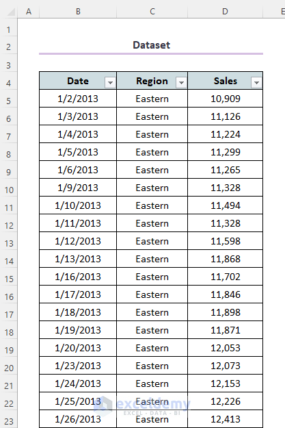
The following dataset contains daily sales by region. The Date field contains the dates for the entire year excluding weekends, the Region field contains the region (Eastern, Southern, or Western), and the Sales field contains the sales amount.
The following dataset shows the Pivot Table created from this data. The Date field is in the Rows area, and the dates have been grouped into months. The Region field is placed in the Columns area. The Sales field has been placed in the Values area.
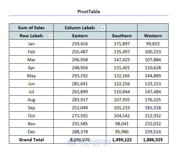
We can easily interpret a Pivot Table rather than raw data. But the easiest way to spot trends is by using the PivotChart
Method 1 – Utilizing the PivotTable Analyze Feature to a Create Chart from a PivotTable
Step 1: Working with the PivotTable Analyze Option
- Select any cell in an existing PivotTable.
- Choose PivotTable Analyze.
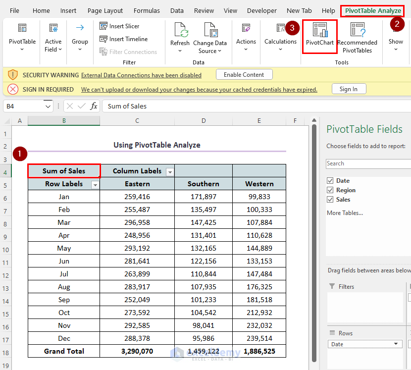
- An Insert Chart window will appear.
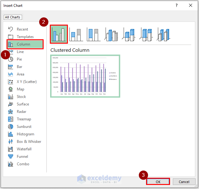
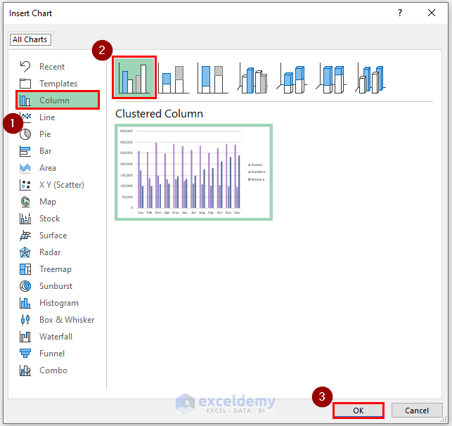
Step 2: Using an Insert Chart Dialogue Box
- Select Column in the Insert Chart
- Click the Clustered Column chart option shown in the picture.
- Click OK.
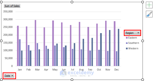
Our PivotChart output will be like this.
The legends of Region and Date are in tabular format. Select various options from these tables to get customized charts.
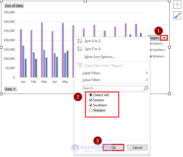
- To get the customized chart, click on Region.
- Select or unselect any of the options of the Region. We have unselected the Western option (i.e., our chart will only be based on Sales in the Eastern and Southern regions).
- Click OK.
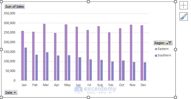
- Our customized chart will look like this.
Read More: How to Edit Pivot Chart in Excel
Method 2 – Using the Insert Option to Create a PivotChart from a PivotTable
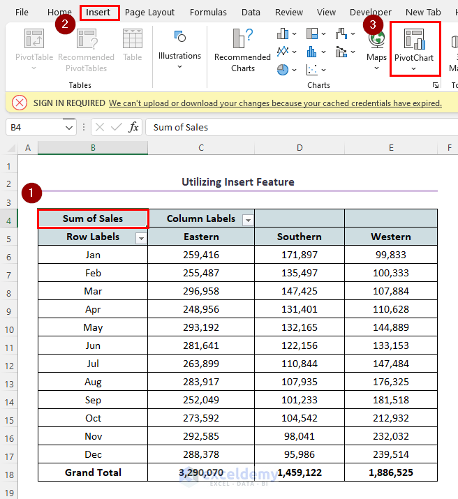
Step 1: Working with the INSERT Option
- Select any cell on the table > go to Insert > choose PivotChart.
- An Insert Chart window will appear.
Step 2: Create a PivotChart
- Select Column in the Insert Chart.
- Click the Clustered Column chart option shown in the picture.
- Click OK.
- We’ll get our PivotChart like this.
- The legends of Region and Date are in tabular format. Select various options from these tables to get customized charts.

Read More: How to Use Pivot Chart in Excel
Create a Pie Chart from the Pivot Table
Steps:
- Click any cell in the table. Here, it is the Sum of Sales.
- Go to Insert > click the drop-down bar of pie charts > select the specified 2-D Pie
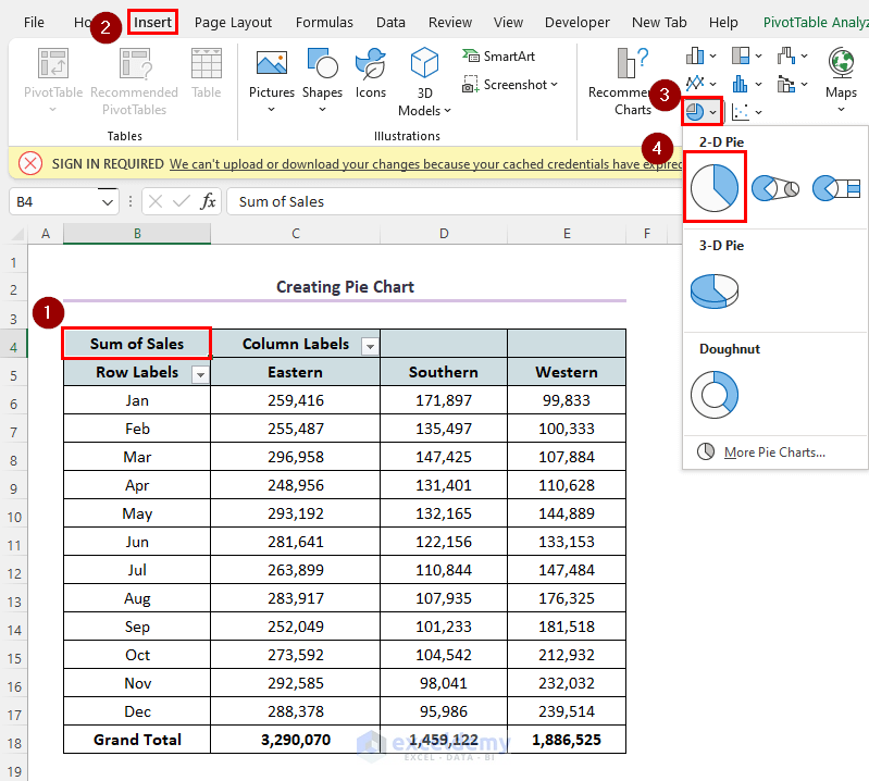
- We’ll see our pie chart like this.
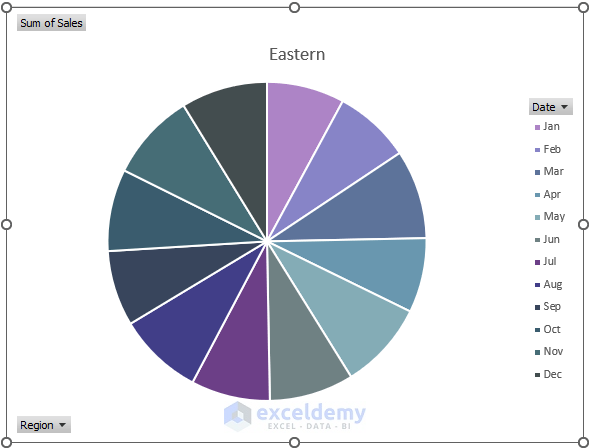
This chart doesn’t contain Sales of all Eastern, Southern and Western regions. So actually, this chart is not practical.
Eventually, we need to adopt another way through which this problem is solved.
- Select one cell in the table > go to Insert > click the drop-down bar of pie charts > select More Pie Charts.
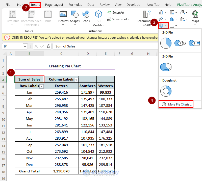
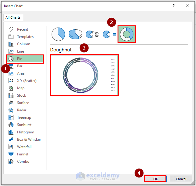
- An Insert Chart window will appear.
- Choose Pie > Select the pictures of the Doughnut chart shown in the image below.
- Click OK.
- We’ll get the chart like this.
- Right-click on the smallest e. innermost circle > select Format Data Series.
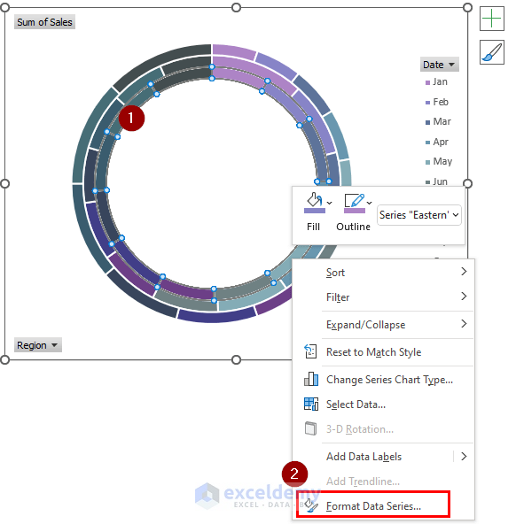
- A Format Data Series window will appear.
- Change the Doughnut Hole Size to 0%.
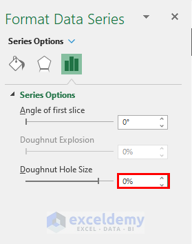
- The shape of the chart is changed like this.
- Right-click the sign shown in the picture > click Data Labels.
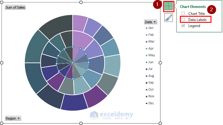
All the data will be added to the chart.
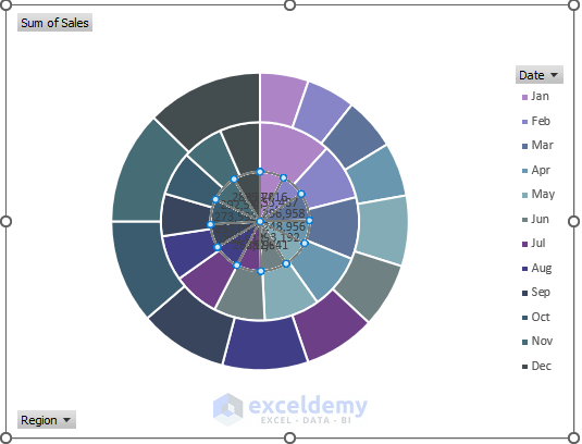
The main problem here is that we have not arranged the data according to their specified places. We need to reorder the data manually. You can rearrange the data inside the chart after creating the pie chart.
Read More: Use Excel VBA to Create Chart from Pivot Table
Things to Remember
- A PivotTable and a PivotChart are joined in a two-way link. If we make any kind of structural or filtering changes to one, we actually have changed the other by default.
- When we activate a PivotChart, the PivotTable Fields task pane will be changed to the PivotChart Fields task pane. In the PivotChart Task pane, Legend (Series) replaces the Columns area, and Axis (Category) replaces the Rows area, and Values are the same for both task panes.
- The field buttons in a PivotChart contain the same controls as the PivotChart’s field headers. These controls allow us to filter the data we display in the PivotTable and PivotChart. If we make changes to the PivotChart using these buttons, PivotTable also displays those changes.
- To move the PivotChart to a different worksheet (or to a Chart Sheet), choose PivotChart Tools ➪ Analyze ➪ Actions ➪ Move Chart.
- It is possible to create multiple PivotCharts from a PivotTable. We can manipulate and format the charts separately. However, all the charts display the same data.
- If we select a normal chart, then it will show the icons to the right: Chart Elements, Chart Styles, and Chart Filters. In contrast, a pivot chart does not display the Chart Filters
- Slicers and Timelines also work with PivotCharts.
- We can choose Page Layout ➪ Themes ➪ Themes to change the workbook theme. Our PivotTable and PivotChart will both use the new theme.
Download Practice Workbook
Related Articles
- Types of Pivot Charts in Excel
- How to Refresh Pivot Chart in Excel
- Data Labels in Excel Pivot Chart
- Difference Between Pivot Table and Pivot Chart in Excel

