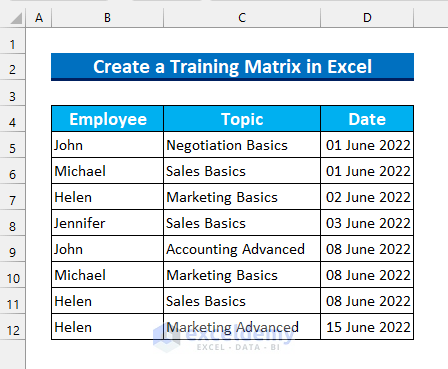
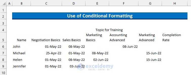
To demonstrate our methods for creating a training Matrix in Excel, we’ll use the following dataset with 3 columns: “Employee”, “Topic”, and “Date”.
Watch Video – Create a Training Matrix in Excel
What Is Training Matrix?
This is basically a table to keep track of employee training programs, which helps the managers of a company decide how many employees need training and how much, assisting in the development of an employee. The main elements of a Training Matrix are the Name, Training Topic, Relevant Dates, and some Calculations. You can optionally include Employee ID, Supervisor, and Working Department.
Method 1 – Using PivotTable
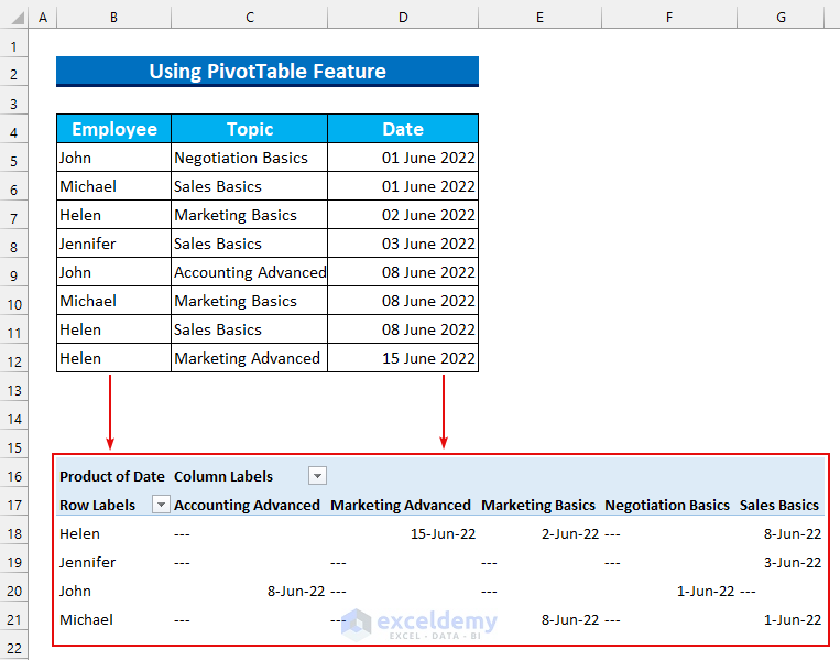
Here, we have a dataset of the employees’ training schedules. We’ll import that data into a PivotTable, then format it using PivotTable options.
Steps:
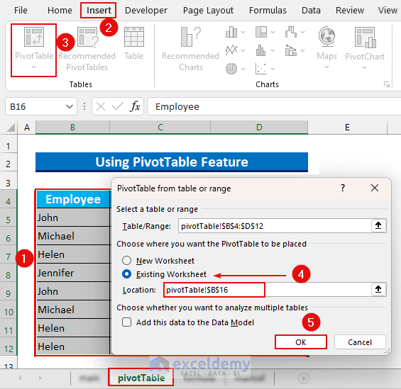
- Select the cell range B4:D12.
- From the Insert tab >>> select PivotTable.
- Select Existing Worksheet and cell B16 as the output location.
- Press OK.
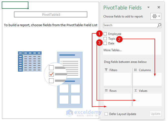
The PivotTable Fields dialog box will open.
Move these Fields:
-
- Employee to Rows.
- Topic to Columns.
- Date to Values.
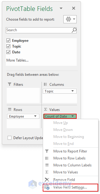
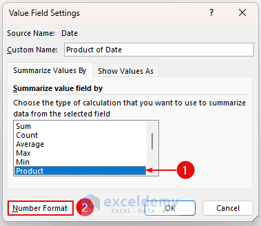
- Select “Count of Date”.
- Select “Value Field Settings…”.
A dialog box will appear.
- Select Product from the “Summarize value field by” section.
- Click on Number Format.
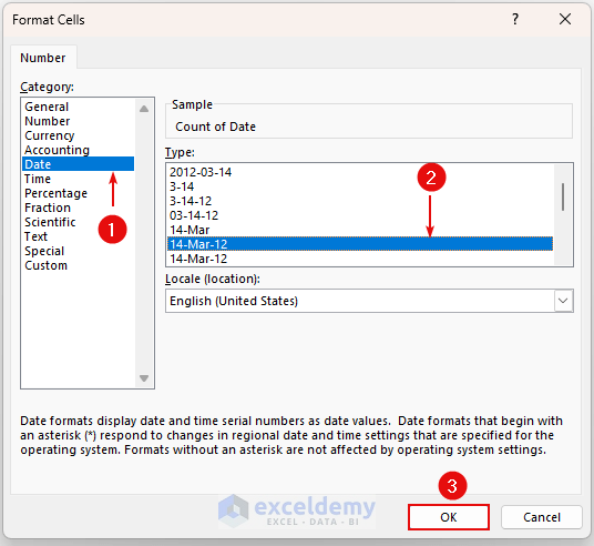
- Select Date from the Category section and enter “14-Mar-22”.
- Press OK.
Now we’ll get rid of the Grand Total from the PivotTable.
- Select the PivotTable.
- From the PivotTable Analyze tab, select Options.
A dialog box will appear.
- From the “Totals & Filters” tab deselect both options under Grand Totals.
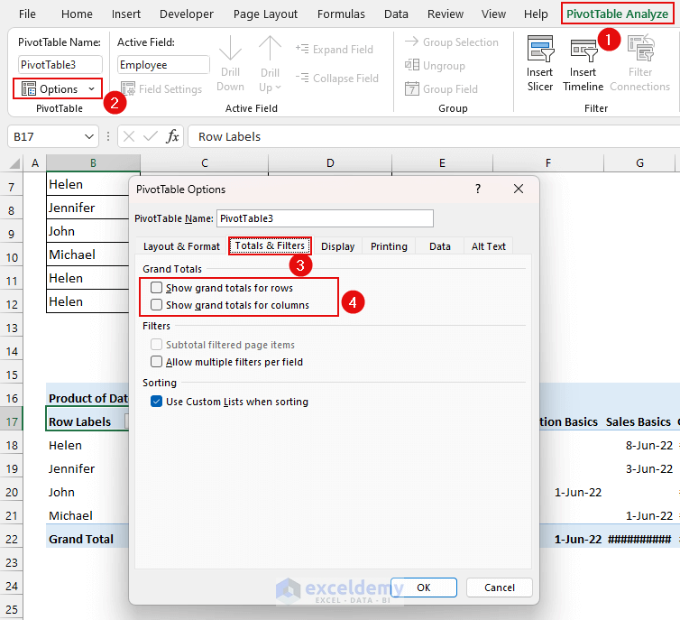
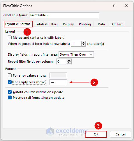
- Under the “Layout & Format” tab, put three dashes ( “—”) for empty cells.
- Click OK.
Our Training Matrix will be generated from our dataset.
Method 2 – Using Combined Formulas
We’ll use the same dataset and the UNIQUE, TRANSPOSE, IFERROR, INDEX, and MATCH functions to create a Training Matrix here.
The UNIQUE function is only available in Excel 2021 and Office 365 versions.
Steps:
- Enter the following formula in cell B18:
=UNIQUE(B5:B12)This function returns the unique value from a range. There are 4 unique names in our defined range.
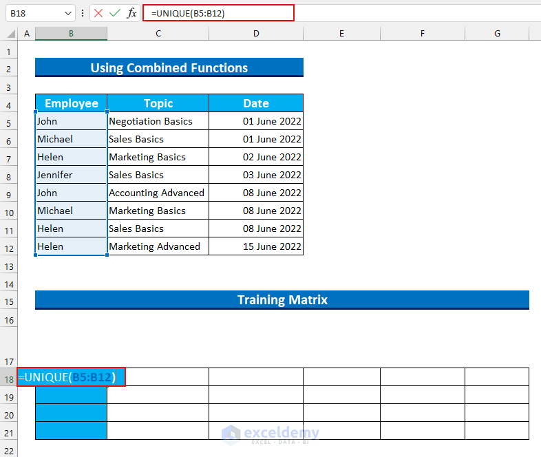
- Press ENTER.
This formula will AutoFill, as it’s an array formula.
- Enter this formula in cell C17:
=TRANSPOSE(UNIQUE(C5:C12))We’re again finding the unique values here. As we want the output to be in the horizontal direction, we added the TRANSPOSE function.
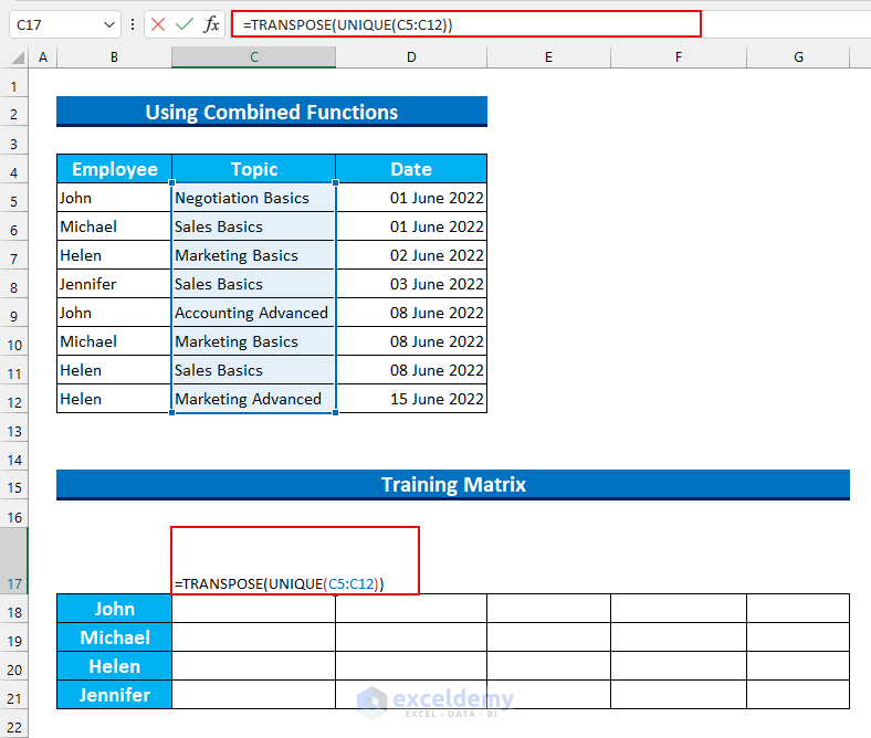
- Press ENTER.
We’ll see the unique values in the horizontal direction here.
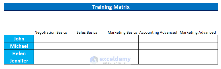
Now we’ll input the dates in the respective fields.
- Enter the following formula in cell C18:
=IFERROR(INDEX($D$5:$D$12,MATCH(1,INDEX(($B$5:$B$12=$B18)*($C$5:$C$12=C$17),),0)),"")Formula Breakdown
- MATCH(1,INDEX(($B$5:$B$12=$B18)*($C$5:$C$12=C$17),),0)
- Output: 1.
- This portion returns the row number for our INDEX function. Inside this portion, there is another INDEX function, which will check how many cells have values from cells B18 and C17.
- Our formula reduces to -> IFERROR(INDEX($D$5:$D$12,1),””)
- Output: 44713.
- This value represents the date “01 June 2022”. Our lookup range is D5:D12. Within that range, we’ll return the value of the first cell D5.
- Our value is returned.
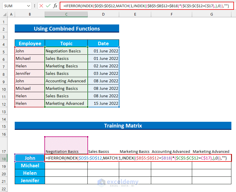
- Press ENTER.
- Use the Fill Handle to AutoFill that formula downwards and then towards the right.
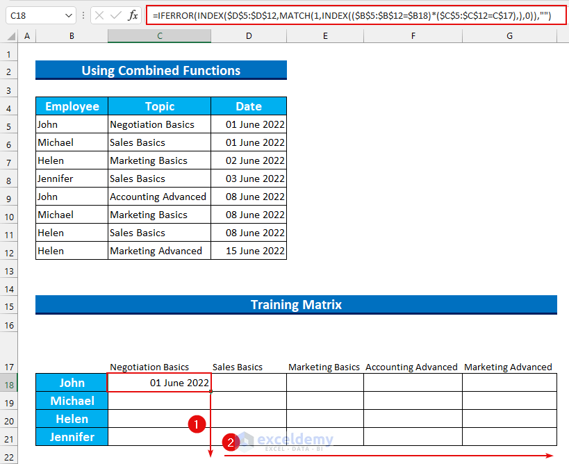
We’ll have output similar to this:
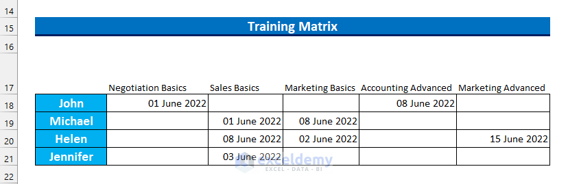
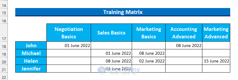
Finally, add some formatting to complete our Training Matrix.
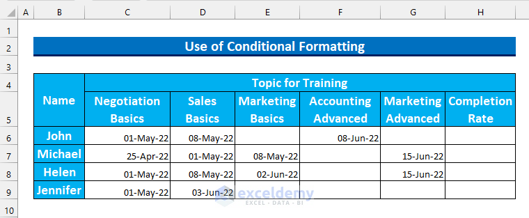
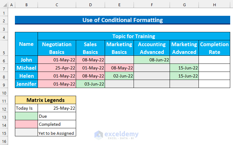
Method 3 – Using Conditional Formatting
Here we’re going to create a Training Matrix from scratch. Then we’ll add Conditional Formatting to it. Finally, we’ll use the COUNT and COUNTIF functions to add percentage completion in our Matrix.
Steps:
- Enter the following data on the Excel Sheet:
- Name of the Employee.
- Topics for Training.
- Relevant Dates.
- Completion Rate column (we’ll add a formula here).
- Format the cells.
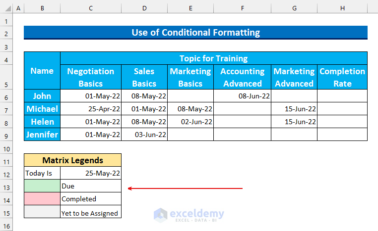
- Add Legends for the Matrix.
Now we’ll add Conditional Formatting to the Matrix.
- Select the cell range C6:G9.
- From the Home tab, select Conditional Formatting, then select “New Rule…”.
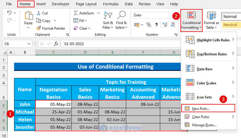
A dialog box will appear.
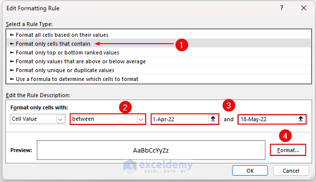
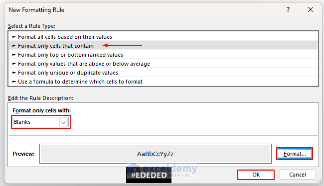
- Select “Format only cells that contain” under Rule type.
- Select “between” and put the date range from “1-Apr-22” to “18-May-22”.
- Press Format.
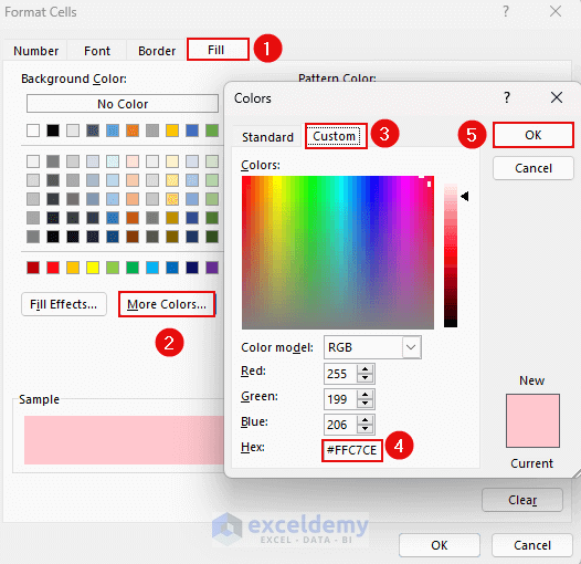
- Select “More Colors…” from the Fill tab.
- From Custom, enter “#FFC7CE” in Hex.
- Click OK.
- Click Apply.
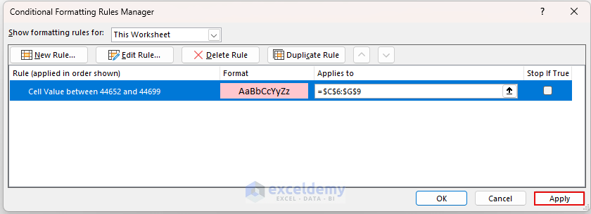
Conditional Formatting is applied to the dates.

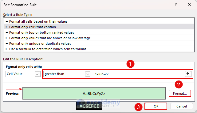
- Similarly, we can add the Green color for future dates.
- And, the Gray color for the blank cells.
The final step should look like this after applying all the formatting. Use the formatting in the order given, else the Gray color may not be visible here.
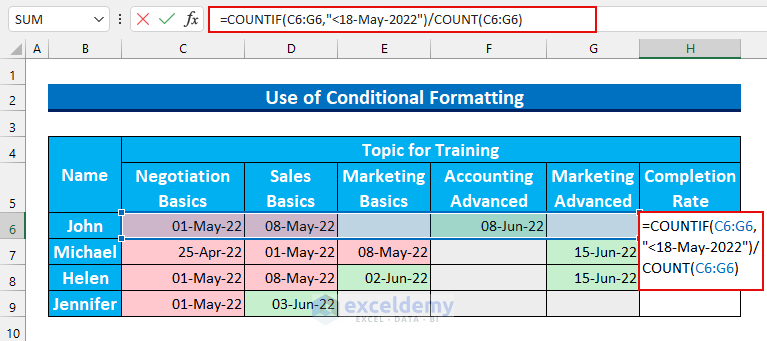
Now we’ll add a formula to calculate the training completion percentage.
- Enter the following formula in cell H6.
=COUNTIF(C6:G6,"<18-May-2022")/COUNT(C6:G6)Formula Breakdown
- With the COUNTIF function, we’re finding the number of cells that have dates before “18 May 2022”. Before this date, the employees have their completed training.
- Then we’re counting the number of non-blank values in our range.
- And then we’re dividing these to calculate the percentage of completion.
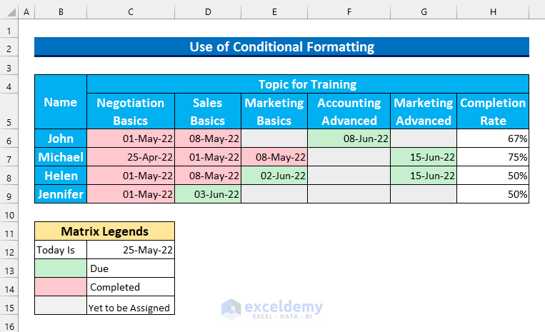
- Press ENTER.
We’ll get almost 0.67 as our output, which is 67%. This value is the percentage of training scheduled for and completed by an employee.

- AutoFill the formula and change the number formatting to show the percentage.
<< Go Back to | Excel for Math | Learn Excel
Get FREE Advanced Excel Exercises with Solutions!

Thanks a lot
You are welcome. I am glad that this article was useful to you.