The steps for creating a risk matrix:
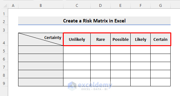
- Define Probability Criteria for an Event
- List the different possibilities or likelihoods of an event occurring. These could range from very unlikely to almost certain. You can enter these possibilities in cells C4:G4. If needed, you can also list them in a column.
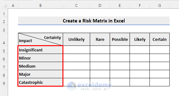
- Set Severity Criteria for an Event
- Create a list of the potential magnitudes that events can cause. For instance, an event might have severe consequences for the business market or a catastrophic impact on the economy. Use impact labels such as insignificant, minor, medium, major, or catastrophic. Place these labels in cells B5:B9.
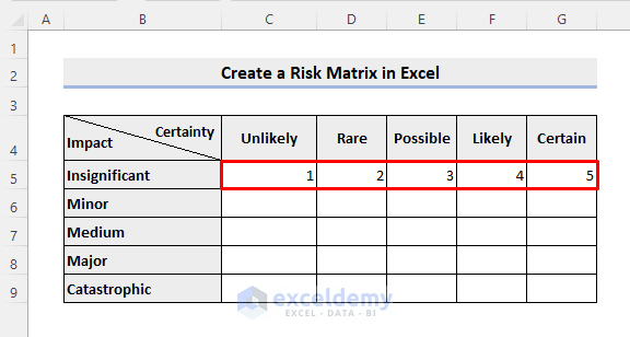
- Assign Numeric Values to Probability
- Assign numbers from 1 to 5 to represent the different possibilities of the event (from Unlikely to Certain). Enter these values in cells C5:G5.
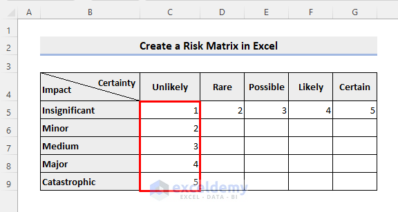
- Assign Numeric Values to Severity
- Similarly, assign numbers from 1 to 5 to represent the severity labels (from Insignificant to Catastrophic). Place these values in cells C5:C9.
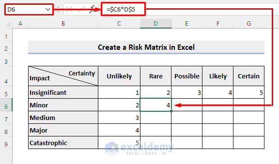
- Create the Formula
- In cell D6, enter the following formula (which contains mixed references)
=$C6*D$5
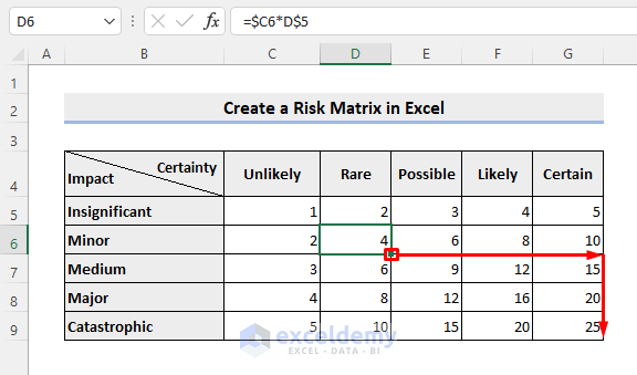
- Fill the Risk Matrix
- Drag the Fill Handle icon to the right and then downward to populate the matrix elements. Alternatively, you can drag it downward first and then to the right.
- Apply Conditional Formatting
- To enhance readability, consider applying conditional formatting to color-code the matrix elements based on their values.
Retrieving Values from a Risk Matrix in Excel
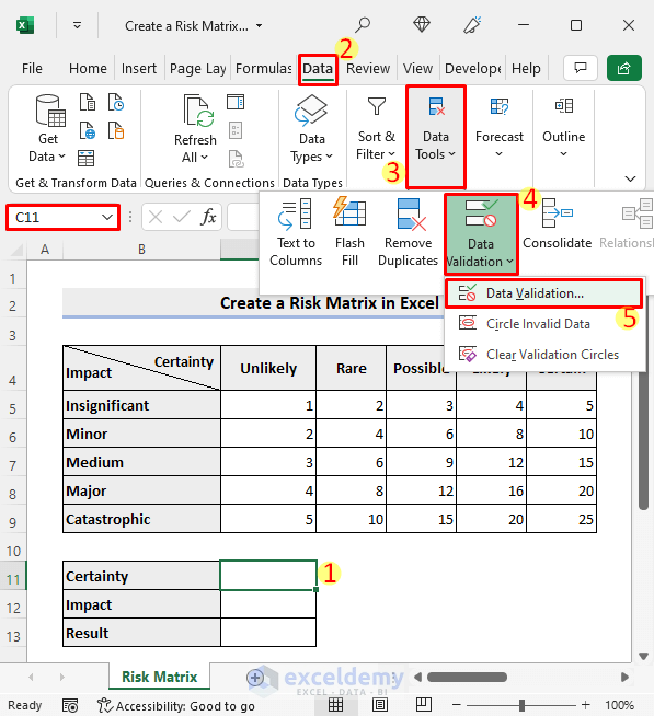
- Create Dropdown Lists
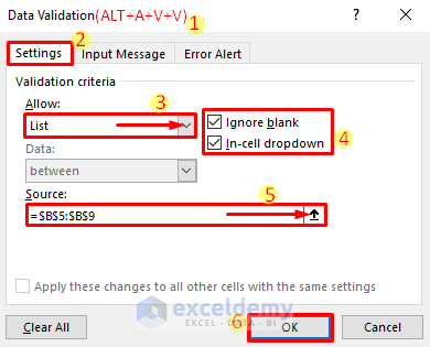
- Select cell C11. This cell will be used for the likelihood of the event. Then, follow these steps:
- Go to the Data tab.
- Click on Data Validation or press ALT + A + V + V to open the Data Validation window.
- Select cell C11. This cell will be used for the likelihood of the event. Then, follow these steps:
-
-
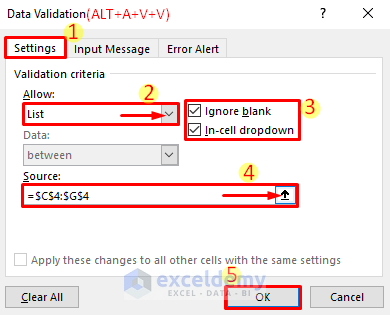
- Choose List as the first validation criteria from the dropdown list.
- Check both Ignore blank and In-cell dropdown options.
- Enter C4:G4 as the source range using the upward arrow.
- Click OK.
-
-
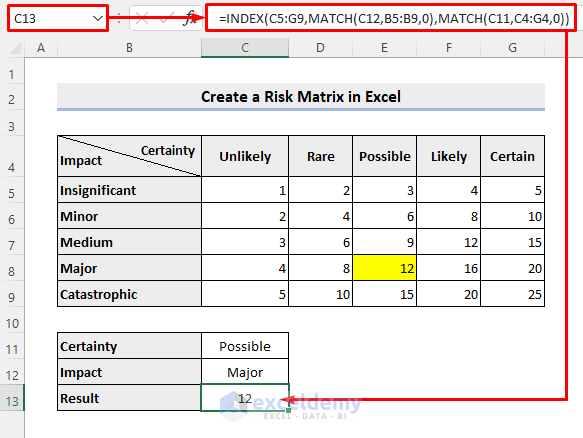
- Create another dropdown list for the impact labels in cell C12. The source range for this dropdown will be B5:B9.
- Retrieve Values Using the Formula
- After selecting likelihood and impact labels from the dropdown lists in cells C11 and C12, enter the following formula in cell C13:
=INDEX(C5:G9,MATCH(C12,B5:B9,0),MATCH(C11,C4:G4,0))
- How the Formula Works
- The INDEX function returns a value or reference from the intersection of a specific row and column within a given range (here, C5:G9).
- The MATCH function finds the relative position of an item in an array that matches a specified value in a specified order.
- MATCH(C12,B5:B9,0) returns the row number (output: 4).
- MATCH(C11,C4:G4,0) returns the column number (output: 3).
- The final result is the value from cell E8 (row 4, column 3).
Things to Remember
- Correct Formula Entry:
Ensure that the formula with mixed references is entered accurately. If it’s not, copying the formula to adjacent cells may result in incorrect or erroneous values.
- Conditional Formatting for Clarity:
Consider using conditional formatting to highlight matrix elements based on their associated risks. This will enhance the matrix’s presentation and make it easier to understand.
Download Practice Workbook
You can download the practice workbook from here:
<< Go Back to Excel for Math | Learn Excel
Get FREE Advanced Excel Exercises with Solutions!
