In an Eisenhower Matrix, we will have two parts. One part is the data section of the template. The data section will contain two parameters named Important and Urgent. We will set two values Yes or No with Data Validation to fix the level of importance and urgency. Another one is the Eisenhower box. This box will consist of four quadrants. Each quadrant will portray a combination of the importance and urgency of our task. Basically, the four combinations of importance and urgency that the four quadrants represent are:
- Important – Urgent
- Important – Not Urgent
- Not Important – Urgent
- Not Important – Not Urgent
So, in the first step, we will create the data section. Then, in the second step, we will create the Eisenhower box.
Step 1 – Create Data Section of Eisenhower Matrix Template
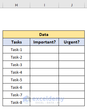
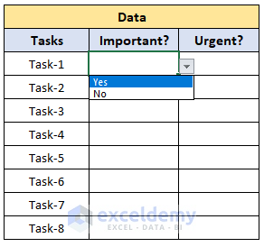
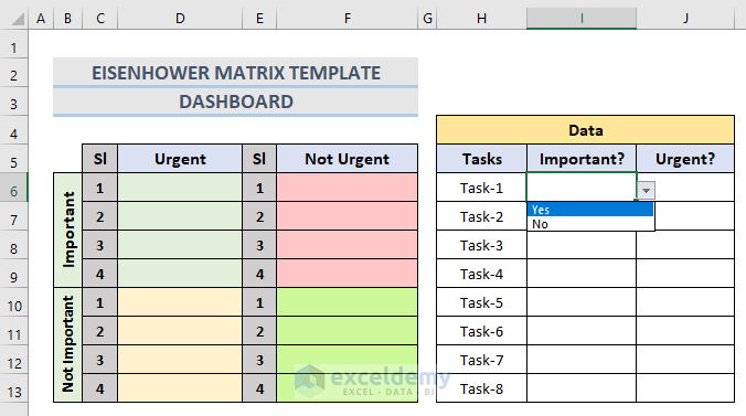
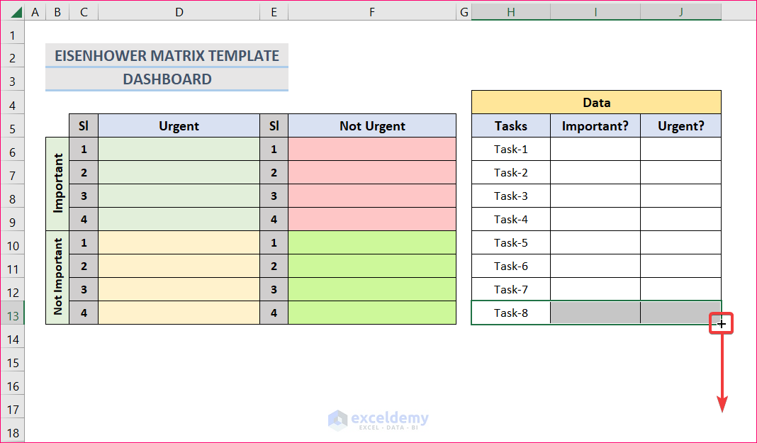
- Make a chart in cell range (H4:J13). Use the headings like the following image.
- Enter the name of the tasks in the Tasks column.
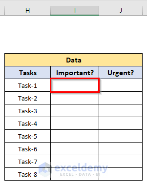
- Select cell I6.
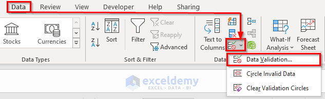
- Go to the Data tab.
- Select the option Data Validation from the Data Validation drop-down menu.
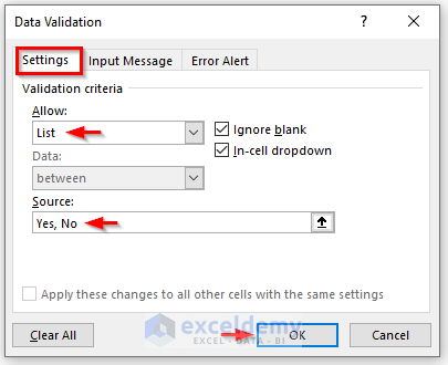
- A new dialogue box named ‘Data Validation’ will open.
- Go to the Settings tab.
- From the Allow section, select the option List from the dropdown menu.
- Type the options Yes and No in the Source field.
- Click on OK.
- We can see a Data Validation dropdown in cell I6. If we click on the dropdown icon of cell I6, the two options Yes and No will be available.
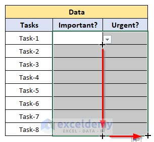
- Drag the Fill Handle tool from cell I6 to I13.
- Drag the Fill Handle tool horizontally from cell I13 to J13.
- Finally, we get a Data Validation dropdown in all the cells from the range (I6:J13). So, we can express the level of importance and urgency of our tasks by selecting the options Yes or No.
Step 2 – Make Eisenhower Box
In the second step, we will create the part Eisenhower box of an Eisenhower matrix in Excel. Once we select some values for a task in the Data section, the task will automatically appear in the Eisenhower matrix box based on importance and urgency.
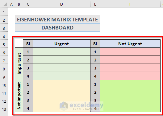
- Create a chart in the cell range (B5:F13) based on the image below, with enough space to fit half the tasks in each sector. You can format it however you like.
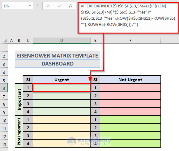
- Select cell D6.
- Insert the following formula in that cell:
=IFERROR(INDEX($H$6:$H$13,SMALL(IF((LEN($H$6:$H$13)<>0)*($I$6:$I$13="Yes")*($J$6:$J$13="Yes"),ROW($H$6:$H$13)-ROW($H$5),""),ROW(H6)-ROW($H$5))),"")- Press Enter.
- Drag the Fill Handle from cell D6 to D9.
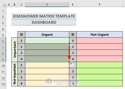
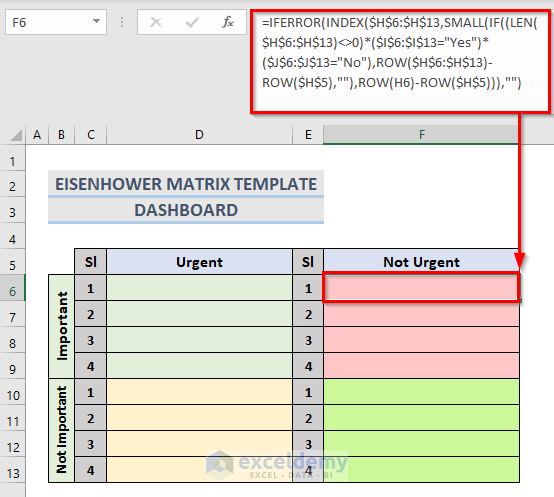
- Select cell F6 and insert the following formula in that cell:
=IFERROR(INDEX($H$6:$H$13,SMALL(IF((LEN($H$6:$H$13)<>0)*($I$6:$I$13="Yes")*($J$6:$J$13="No"),ROW($H$6:$H$13)-ROW($H$5),""),ROW(H6)-ROW($H$5))),"")- Hit Enter.
- Pull the Fill Handle tool from cell F6 to F9.
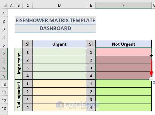
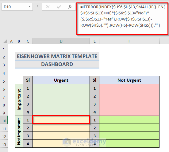
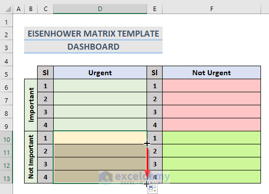
- Select cell D10.
- Enter this formula in the cell:
=IFERROR(INDEX($H$6:$H$13,SMALL(IF((LEN($H$6:$H$13)<>0)*($I$6:$I$13="No")*($J$6:$J$13="Yes"),ROW($H$6:$H$13)-ROW($H$5),""),ROW(H6)-ROW($H$5))),"")- Press Enter.
- Drag the Fill Handle tool from cell D10 to D13.
- Select cell F10. Paste the following formula in that cell:
=IFERROR(INDEX($H$6:$H$13,SMALL(IF((LEN($H$6:$H$13)<>0)*($I$6:$I$13="No")*($J$6:$J$13="No"),ROW($H$6:$H$13)-ROW($H$5),""),ROW(H6)-ROW($H$5))),"")- Press Enter.
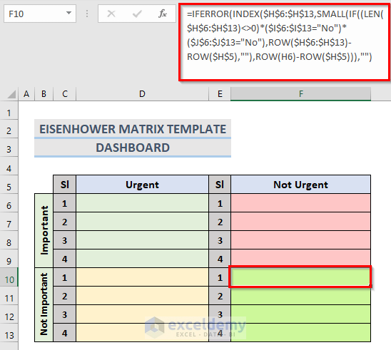
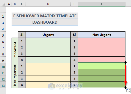
- Drag the Fill Handle tool from cell F10 to F13.
- The process of making an Eisenhower box is finished now.
How Does the Formula Work?
- ROW($H$6:$H$13)-ROW($H$5): In this part, the ROW function returns a numeric value for each task in cells (I6:I13).
- LEN($H$6:$H$13): Here, the LEN function returns the lengths of each text from cells (H6:H13).
- IF((LEN($H$6:$H$13)<>0)*($I$6:$I$13=”Yes”)*($J$6:$J$13=”Yes”),ROW($H$6:$H$13)-ROW($H$5),””): Suppose in a particular row both values from cell (I6:I13) and (J6:J13) is Yes. Then, the above part of the formula with the IF function will return the text from the range (H6:H13) in that row.
- SMALL(IF((LEN($H$6:$H$13)<>0)*($I$6:$I$13=”Yes”)*($J$6:$J$13=”Yes”),ROW($H$6:$H$13)-ROW($H$5),””): Here the SMALL function returns the lowest matching value for each array.
- (INDEX($H$6:$H$13,SMALL(IF((LEN($H$6:$H$13)<>0)*($I$6:$I$13=”Yes”)*($J$6:$J$13=”Yes”),ROW($H$6:$H$13)-ROW($H$5),””): Lastly, this formula wit the INDEX function looks for matched values in the array (H6:H13) and returns them in cell D6.
- IFERROR(INDEX($H$6:$H$13,SMALL(IF((LEN($H$6:$H$13)<>0)*($I$6:$I$13=”Yes”)*($J$6:$J$13=”Yes”),ROW($H$6:$H$13)-ROW($H$5),””),ROW(H6)-ROW($H$5))),””): This part returns the final result in cell D6. If the value gets an error the IFERROR function returns blank.
Features of Eisenhower Matrix Template in Excel
We will create the same template that we created in earlier steps. To illustrate the process we will follow the below steps.
Steps:
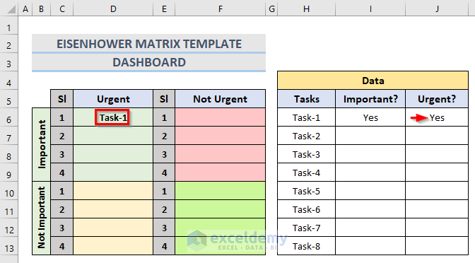
- Select importance level Yes from the dropdown menu of cell I6.
- Select the value Yes in cell J7.
- As a result, Task-1 automatically appears in the first quadrant of the Eisenhower box. It means Task-1 is both important and urgent.
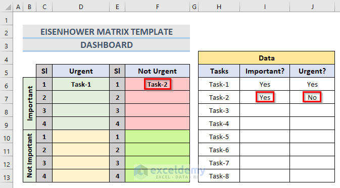
- For Task-2, select the value Yes for the importance level in cell I7. But, select the value No for urgency level in cell J7.
- So, Task-2 appears in the 2nd quadrant. This means that Task-2 is important but not urgent.
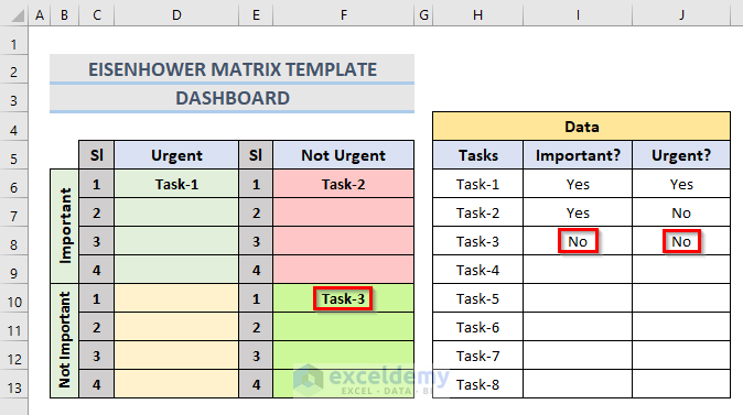
- For Task-3, choose No for both cells I8 and J8.
- We can see Task-3 in the fourth quadrant.
Download Free Template
You can download the template from here.
<< Go Back to Excel for Math | Learn Excel
Get FREE Advanced Excel Exercises with Solutions!

I don’t see a link to download the “practice workbook” that comes with this article.
Please forward.
Thank you,
Hello, Mary Visco! The downloadable file has been sent to your gmail address. If you can’t find the mail in inbox then please look for it in spam folder. Best regards!
Hello,
I am trying this “How to make”, but the formula for the Matrix does not work.
=IFERROR(INDEX($H$6:$H$13,SMALL(IF((LEN($H$6:$H$13)0)*($I$6:$I$13=”Yes”)*($J$6:$J$13=”Yes”),ROW($H$6:$H$13)-ROW($H$5),””),ROW(H6)-ROW($H$5))),””)
I think the problem starts here
IF((LEN($H$6:$H$13)0)*($I$6:$I$13=”Yes”)*($J$6:$J$13=”Yes”),ROW($H$6:$H$13)-ROW($H$5),””)
Any suggestions? Working with Microsoft 365.
Hi KARLHEINZ,
Looks like you have missed the <> symbol in the SMALL(IF((LEN($H$6:$H$13)0) portion of the formula. The correct formula should be this:
SMALL(IF((LEN($H$6:$H$13)<>0)
I hope this solves your problem. Please let us know if you face any other issues.
Hello,
I have tried the download version and to make my own and neither will add the task when set to yes or no on the matrix.
I have copied the formula on this site into the cells and drag copied down for each section of the matrix the specific code, but still no results.
Any suggestions?
Thanks!
Hello JC,
Thanks for your comment. I am replying to you on behalf of ExcelDemy. The downloaded file works for me.
You can follow the steps from the Feature of Eisenhower Matrix Template in Excel section. If it still doesn’t work then check if all cells contain the formula in the Eisenhower Matrix.
And, while making your own Eisenhower Matrix, check if you are applying for the same range as in this article. If not, change your ranges accordingly in the formula.
Lastly, if you are using an older version of Microsoft Excel then press Ctrl + Shift + Enter while entering the formula.
I hope this will help you to solve your problem. If none of these works then you can let us know at [email protected] with your Excel file and problem details. We will try our best to solve your problem.
Regards
Mashhura
ExcelDemy
Hello,
I am using two sheets. One sheet has the info (Task E7, Priority B7(High, Medium, Low)) and the second sheet will have the prioritization matrix.
How do i reference the formula from another sheet? Or what would be the formula in this case? Thank you.
Hello SEAN,
Here, we have listed the following tasks in a sheet which we will classify according to their importance and urgency.
• For creating drop-down lists for each of the cells in range C5:D12, we have opened the Data Validation dialog box.
• In the Source box, type High, Medium, Low.
Then, we selected the following values for the tasks in the Task sheet.
In another sheet named Matrix, we have created the following template.
• For the portion of High Important and High Urgent use the following formula in cell D5, press ENTER, and use the AutoFill feature up to cell D8.
=IFERROR(INDEX(Task!$B$5:$B$12,SMALL(IF((LEN(Task!$B$5:$B$12)<>0)*(Task!$C$5:$C$12="High")*(Task!$D$5:$D$12="High"),ROW(Task!$B$5:$B$12)-ROW(Task!$B$4),""),ROW(Task!B5)-ROW(Task!$B$4))),"")• For the portion of High Important and Medium Urgent use the following formula in cell F5, press ENTER, and use the AutoFill feature up to cell F8.
=IFERROR(INDEX(Task!$B$5:$B$12,SMALL(IF((LEN(Task!$B$5:$B$12)<>0)*(Task!$C$5:$C$12="High")*(Task!$D$5:$D$12="Medium"),ROW(Task!$B$5:$B$12)-ROW(Task!$B$4),""),ROW(Task!B5)-ROW(Task!$B$4))),"")• For the portion of High Important and Low Urgent use the following formula in cell H5, press ENTER, and use the AutoFill feature up to cell H8.
=IFERROR(INDEX(Task!$B$5:$B$12,SMALL(IF((LEN(Task!$B$5:$B$12)<>0)*(Task!$C$5:$C$12="High")*(Task!$D$5:$D$12="Low"),ROW(Task!$B$5:$B$12)-ROW(Task!$B$4),""),ROW(Task!B5)-ROW(Task!$B$4))),"")• For the portion of Medium Important and High Urgent use the following formula in cell D9, press ENTER, and use the AutoFill feature up to cell D12.
=IFERROR(INDEX(Task!$B$5:$B$12,SMALL(IF((LEN(Task!$B$5:$B$12)<>0)*(Task!$C$5:$C$12="Medium")*(Task!$D$5:$D$12="High"),ROW(Task!$B$5:$B$12)-ROW(Task!$B$4),""),ROW(Task!B5)-ROW(Task!$B$4))),"")• For the portion of Medium Important and Medium Urgent use the following formula in cell F9, press ENTER, and use the AutoFill feature up to cell F12.
=IFERROR(INDEX(Task!$B$5:$B$12,SMALL(IF((LEN(Task!$B$5:$B$12)<>0)*(Task!$C$5:$C$12="Medium")*(Task!$D$5:$D$12="Medium"),ROW(Task!$B$5:$B$12)-ROW(Task!$B$4),""),ROW(Task!B5)-ROW(Task!$B$4))),"")• For the portion of Medium Important and Low Urgent use the following formula in cell H9, press ENTER, and use the AutoFill feature up to cell H12.
=IFERROR(INDEX(Task!$B$5:$B$12,SMALL(IF((LEN(Task!$B$5:$B$12)<>0)*(Task!$C$5:$C$12="Medium")*(Task!$D$5:$D$12="Low"),ROW(Task!$B$5:$B$12)-ROW(Task!$B$4),""),ROW(Task!B5)-ROW(Task!$B$4))),"")• For the portion of Low Important and High Urgent use the following formula in cell D13, press ENTER, and use the AutoFill feature up to cell D16.
=IFERROR(INDEX(Task!$B$5:$B$12,SMALL(IF((LEN(Task!$B$5:$B$12)<>0)*(Task!$C$5:$C$12="Low")*(Task!$D$5:$D$12="High"),ROW(Task!$B$5:$B$12)-ROW(Task!$B$4),""),ROW(Task!B5)-ROW(Task!$B$4))),"")• For the portion of Low Important and Medium Urgent use the following formula in cell F13, press ENTER, and use the AutoFill feature up to cell F16.
=IFERROR(INDEX(Task!$B$5:$B$12,SMALL(IF((LEN(Task!$B$5:$B$12)<>0)*(Task!$C$5:$C$12="Low")*(Task!$D$5:$D$12="Medium"),ROW(Task!$B$5:$B$12)-ROW(Task!$B$4),""),ROW(Task!B5)-ROW(Task!$B$4))),"")• For the portion of Low Important and Low Urgent use the following formula in cell H13, press ENTER, and use the AutoFill feature up to cell H16.
=IFERROR(INDEX(Task!$B$5:$B$12,SMALL(IF((LEN(Task!$B$5:$B$12)<>0)*(Task!$C$5:$C$12="Low")*(Task!$D$5:$D$12="Low"),ROW(Task!$B$5:$B$12)-ROW(Task!$B$4),""),ROW(Task!B5)-ROW(Task!$B$4))),"")Note:
Here, we have used the sheet name Task in all our formulas, if you have any other sheet name, then put this name in the formulas.
Regards
Tanjima Hossain
I’m not able to adjust the ranges in these formulas in order to make a longer reference list without causing an error. Please advise. Thanks
Hello Theo,
Follow these steps to adjust ranges to make a longer list without any error.
1. First, to make the task list longer, select cells H13 through J13. Then drag the fill handle down to add new task.
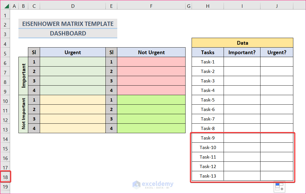
2. In this example, we added five new tasks. Therefore, the new ranges for column H, I and J are H6:H18, I6:I18 and J6:J18 respectively.
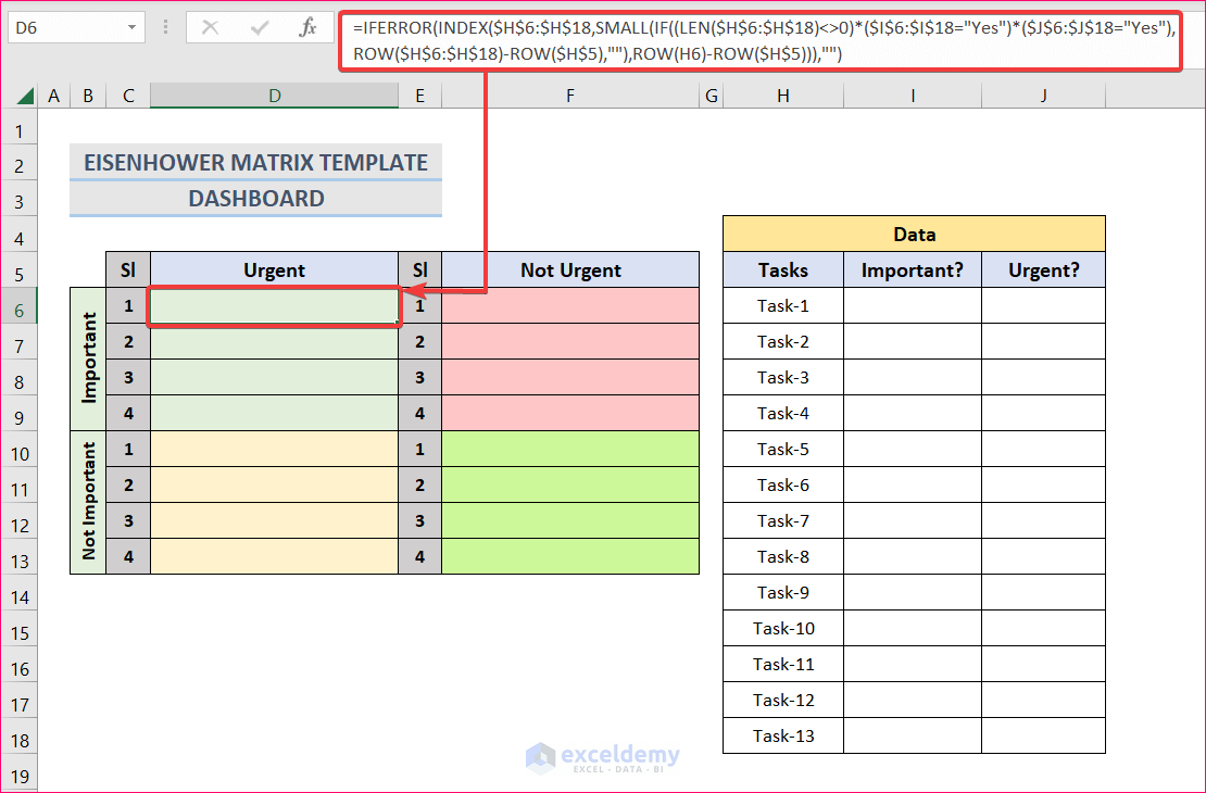
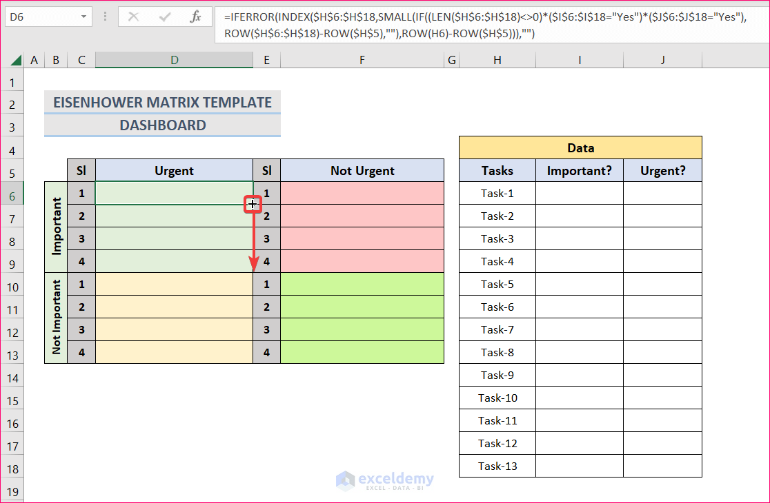
3. Then select cell D6 and change the ranges of H,I and J cells in the formula bar and press Enter. After that, Autofill formula up to cell D9.
4. Similarly, change the formula ranges for other cells as well.
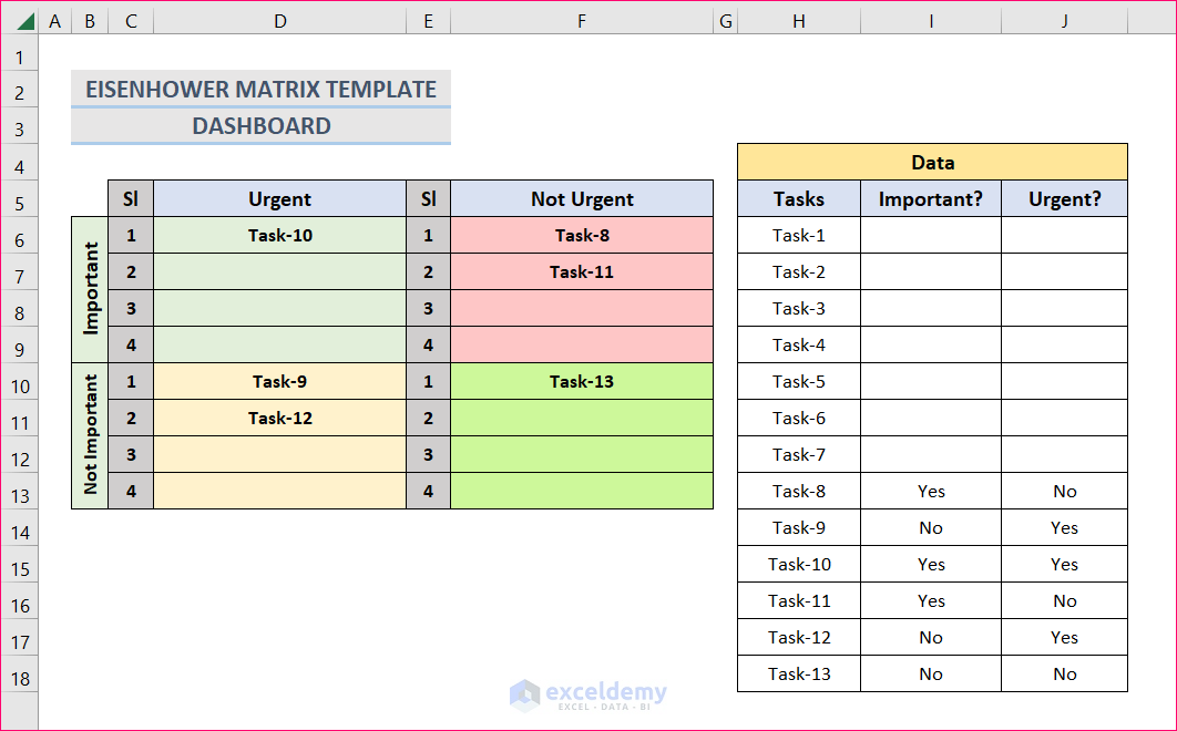
5. Finally, you can see in the following figure that the formula is working properly.
I hope this solves your problem. Please let us know if you face any other issues.
Hello! This has worked perfectly for my worksheet – thank you! My worksheet also contains a column that marks the status of the task (ongoing, on hold, completed, cancelled). I’m struggling with coming up with a conditional formatting or additional formula that will remove an item from the Eisenhower box once it has been updated as completed or cancelled within my to do list.
Within my to do list, the conditional formatting comes into play and shades out and places strike through once a task is completed or cancelled. Is there a way to then have the box update to remove those tasks from the quadrants once it recognizes a complete or cancelled?
I hope you need something like this- once you update the status of a work in a column, there will be a strikethrough in the Eisenhower dashboard.
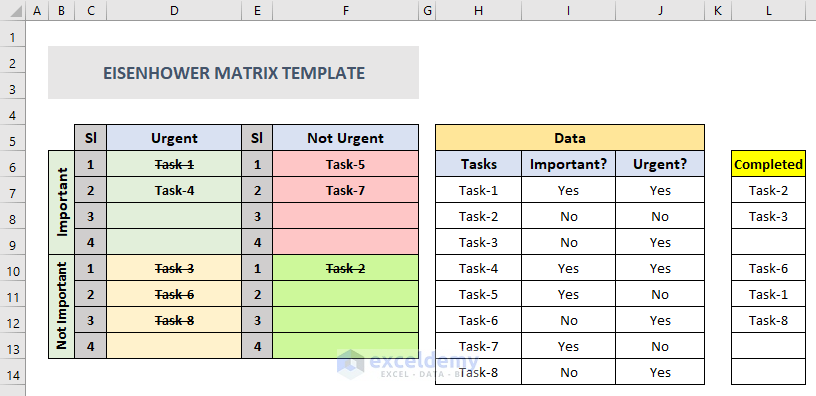
Here is a sample how you can work with it.
You can see that the completed tasks (Task-2, Task-3 etc.) get a strikethrough in the Urgent and Not Urgent columns. For this purpose, we will apply two conditional formatting for two types of work (Urgent and Not Urgent). Select the Urgent range first and then go to Conditional Formatting >> New Rule.
The New Formatting Rule window will appear. Select the option Use a formula to determine which cells to format and type the formula below in the ‘Format values where this formula is true‘ section.
[wpsm_box type="red" float="none" textalign="center"]
=OR(D6=$L$7:$L$14)[/wpsm_box]
After that, click on the Format button.
In the next window, check Strikethrough and click OK.
You will see a preview of how the formatted texts will look like, just click OK.
Finally you will see the Strikethroughs on the Completed Urgent tasks in the Eisenhower dashboard.
Do the same Conditional Formatting procedure for the Not Urgent range. You will get Strikethroughs on Not Urgent Completed tasks.
Why this formulas are not working from second row onwards in my data sheet.
I have copied the formula as mentioned above and in the dedicated cells as instructed, but the same conditioning of data in 2nd row does not even show output.
pls help
Hello DEEP!
From your comment, I think the most possible reason of the error could be inappropriate cell referencing. Please note that these formulas include both absolute and relative cell reference. You may copy paste the formulas, and then adjust the cell references according to your dataset. Hopefully that will solve your issue.
Output:
If you need further assistance regarding this, please feel free to send the Excel file in this email [email protected].
Regards
Hadi Ul Bashar
It still is not working. I will send the excel files to the link provided. Thank you.
Hello Daniel Woods,
To make problem sharing easier we launched ExcelDemy Forum, so that you can upload Excel Files and images of your problem. You can share your workbook in ExcelDemy Forum our expert team will reach out to you.
Regards
ExcelDemy
This is very helpful, I feel like it WHT 8 will need 9n jy next adventure to prioritize my time
What seems to be happening is if you increase the data range, for some reason the chart stops working beyond the original data range. Is there a solve for this?
Hi Mr. Woods, thanks for reaching out. Here’s a quick solution to your problem. Just convert your data range to a table. If you enlarge the data range after that, the formulas will update accordingly and you will get your desired result.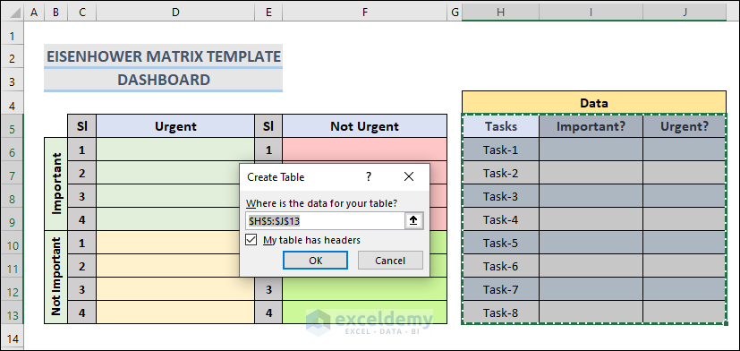
 However, here we made 4 4×1 matrices for different type of works. If you want to insert more tasks, just increase the rows corresponding important and not important tasks. I suggest you to go through the other comments if you haven’t already as you may find them useful.
I’m going to show the solution with images so you can understand this topic easily. First, I’m converting the Data range to a table. Select the marked range and press Ctrl + T to convert this range to a table.
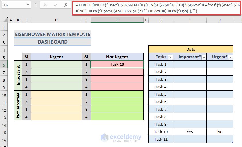
Now, add some rows to the table and insert the type of a task in the additional data range. You will see the task appear in the corresponding cell. Also, notice that the range in the formula updates automatically.
And now it looks like the email doesn’t work either. Is there an email I can reach you to review my templates?
Hello Daniel Woods,
To make problem sharing easier we launched ExcelDemy Forum, so that you can upload Excel Files and images of your problem. You can share your workbook in ExcelDemy Forum our expert team will reach out to you.
Regards
ExcelDemy
Hi i would like to know why my formula is not working. It is right but I cannot see the output of the formula. Can you please help troubleshoot? Thank you so much for your help. I really really appreciate it.
my formula is =IFERROR(INDEX($C$4:$C$30,SMALL(IF((LEN($C$4:$C$30)0)*($D$4:$D$30=”yes”)*($E$4:$E$30=”yes”),ROW($C$4:$C$30)-ROW($C$3),””),ROW($C$4)-ROW($C$3))),””)
Hello SINTA R
Thanks for reaching out and sharing your queries. The formula you have mentioned is almost correct. However, you miss to insert the <> sign somehow in your formula.
You can apply the following formulas:
For Important & Urgent:
=IFERROR(INDEX($C$4:$C$30,SMALL(IF((LEN($C$4:$C$30)<>0)*($D$4:$D$30="Yes")*($E$4:$E$30="Yes"),ROW($C$4:$C$30)-ROW($C$3),""),ROW(C4)-ROW($C$3))),"")For Important & Not Urgent:
=IFERROR(INDEX($C$4:$C$30,SMALL(IF((LEN($C$4:$C$30)<>0)*($D$4:$D$30="Yes")*($E$4:$E$30="No"),ROW($C$4:$C$30)-ROW($C$3),""),ROW(C4)-ROW($C$3))),"")For Not Important & Urgent:
=IFERROR(INDEX($C$4:$C$30,SMALL(IF((LEN($C$4:$C$30)<>0)*($D$4:$D$30="No")*($E$4:$E$30="Yes"),ROW($C$4:$C$30)-ROW($C$3),""),ROW(C4)-ROW($C$3))),"")For Not Important & Not Urgent:
=IFERROR(INDEX($C$4:$C$30,SMALL(IF((LEN($C$4:$C$30)<>0)*($D$4:$D$30="No")*($E$4:$E$30="No"),ROW($C$4:$C$30)-ROW($C$3),""),ROW(C4)-ROW($C$3))),"")OUTPUT OVERVIEW:
Hopefully, you have found your solution. I have also attached the solution workbook for better understanding; good luck.
DOWNLOAD SOLUTION WORKBOOK
Regards
Lutfor Rahman Shimanto
ExcelDemy