Covariance refers to the measurement of how one variable defers to another. The variables do not have to be dependent on one another. The formula for calculating covariance is represented in the following image.
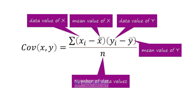
Xi = Data value of the first category
Yi = Data value of the second category
X̄ = Mean data Value of the first category
Ȳ = Mean data Value of the second category
n = Total number of data values
We’ll create two matrices with two categories each and use the covariance command in Excel to calculate the deviations. We’ll use the Data Analysis ribbon from the Data tab to do this.
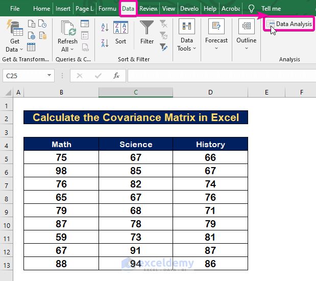
We have a dataset of scores in three subjects.
Step 1 – Apply the Data Analysis Command in Excel
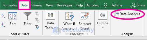
- Click on the Data tab.
- From the Analysis group, select the Data Analysis command.
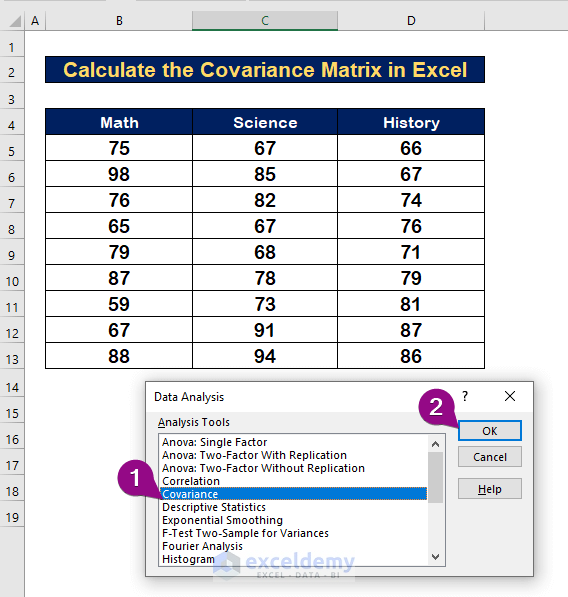
Step 2 – Select the Covariance Option from Analysis Tool
- From the Analysis Tools list, select the Covariance option.
- Click OK.
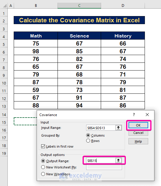
Step 3 – Select the Range to Calculate Covariance Matrix in Excel
- To calculate variance with Math, Science, and History, select the Input Range B4:D13 alongside the Header.
- Select Labels in first row box.
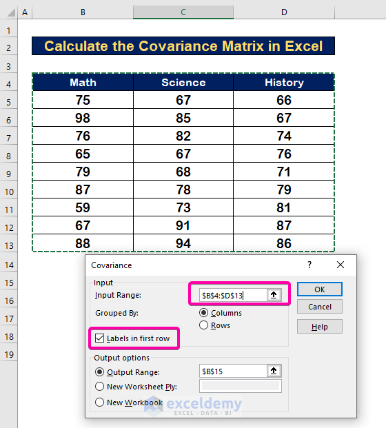
- For Output Range, select any cell (B15).
- Click OK.
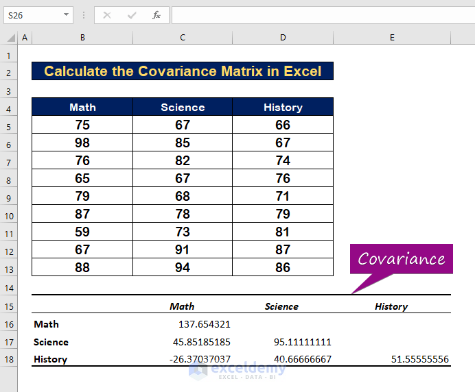
- The covariances will appear as in the image shown below.
How to Interpret the Covariance Matrix in Excel
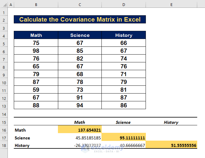
Case 1 – Covariance for a Single Variable
- The variance of Math with its mean is 137.654321.
- The variance of Science is 95.1111.
- The variance of History is 51.5555.
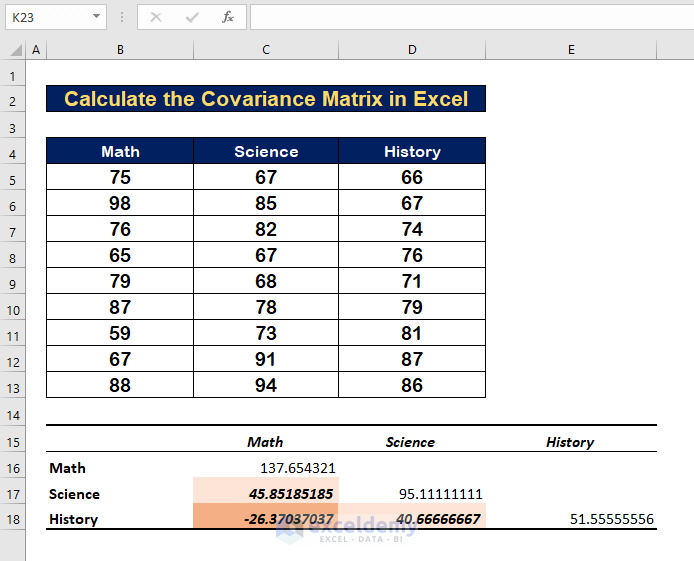
Case 2 – Covariance for Multiple Variables+
- The variance value between Math and Science is 45.85185.
- The variance value between Math and History is -27.3703.
- The variance value between Science and History is 86.66667.
Positive Covariance
The presence of positive covariance indicates that the two variables are proportionate. When one variable rises, the other tends to rise with it. As in our example, the covariance between Math and Science is positive (45.85185), implying that students who perform well in Math also perform well in Science.
Negative Covariance
Negative covariance, in contrast to positive covariance, means that when one variable increases, the other decreases. The covariance between Math and History in our example covariance is negative (-27.3703), indicating that students who score higher in Math will score lower in History.
Notes:
If you cannot find the Data Analysis tool in your Data tab, you may need to activate the Data Analysis ToolPak first.
- Go to Home.
- Click on Options.

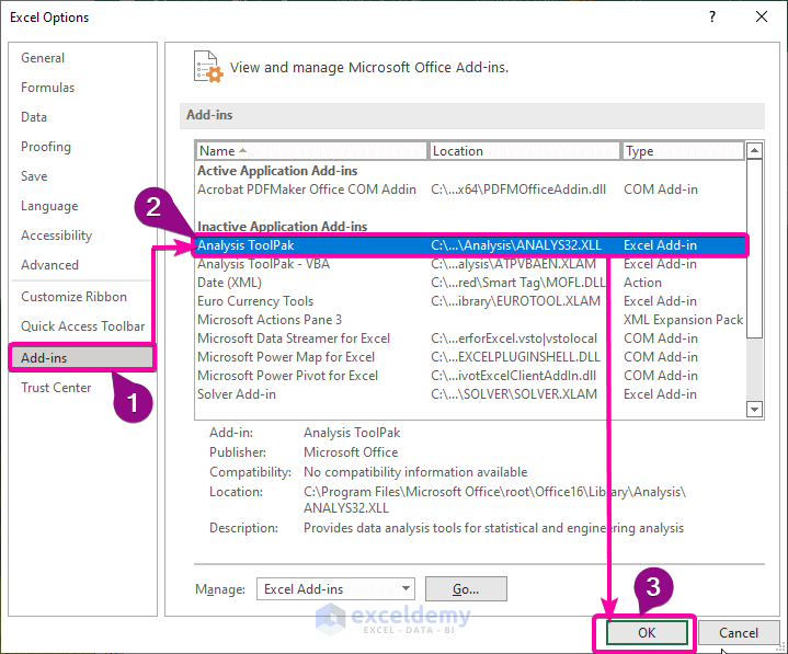
- From Excel Options, select the Add-ins options.
- Click the Analysis ToolPak option.
- Click OK.
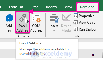
- Go to the Developer tab.
- From Add-ins, click on the Excel Add-ins command.
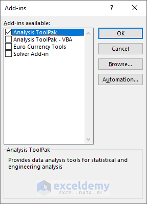
- Select the Analysis ToolPak from the list.
- Click OK to add the Add-in.
- You will find the Data Analysis command in your Data tab.
Download the Practice Workbook
<< Go Back to Excel for Math | Learn Excel
Get FREE Advanced Excel Exercises with Solutions!
