This article illustrates how to apply conditional formatting borders in Excel. Conditional formatting is one of the most useful features in Excel. You can use it to apply borders to cells automatically saving time and effort. Follow the article and you will be able to apply it in 4 useful cases.
Apply Borders in Excel Conditional Formatting: 4 Ways
1. Apply Conditional Formatting with Borders for Non-Blank Cells
Follow the steps below to apply cell borders automatically whenever you enter values.
📌 Steps:
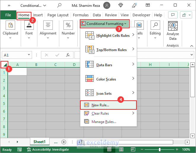
- First, select the desired range to apply the formatting. If you want to apply it to the entire worksheet, click on the downward arrow in the upper-left corner of the first cell. Then select Home >> Conditional Formatting >> New Rule.
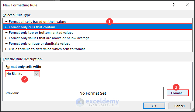
- Next select Format only cells that contain >> Format only cells with >> No Blanks >> Format as shown below.
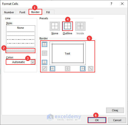
- After that, go to the Border tab from the Format Cells dialog box. Change the line style and color if you want. Now click on the Outline preset or any other border type from the Borders section as required. Click OK After that.
- Finally, enter values in the cells and you will see cell borders added to those cells automatically.
Read More: How to Copy Conditional Formatting to Another Sheet
2. Conditional Formatting with Borders for Non-Empty Rows/Columns
Follow the steps below to apply cell borders automatically to non-empty rows or columns whenever you enter values.
📌 Steps:
- Assume you need to apply a border to the entire row whenever you enter data in cells in column A.
- Then first select the desired range or the entire sheet to apply the formatting. Then go to Home >> Conditional Formatting >> New Rule.
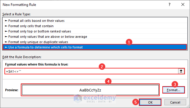
- Next, select Use a formula to determine which cells to format as the rule type. After that, enter the following formula in the formula box.
=$A1<>""- Then click on Format, select the Outline preset, and click OK.
- Finally, enter values in cells in column A and you will see cell borders applied to the corresponding rows.
- If you want to apply a border to the entire row by entering values in any cell, use the following formula instead.
=COUNTA($A1:$XFD1)>0- You can use the following alternative formulas to create new formatting rules to apply cell borders to columns.
=A$1<>""=COUNTA(A$1:A$1043576)>0Read More: How to Copy Conditional Formatting with Relative Cell References in Excel
3. Conditional Formatting with Borders for Groups of Rows/Columns
Follow the steps below to apply cell borders automatically to group rows or columns together based on their values.
📌 Steps:
- Consider the following dataset. Assume you need to apply borders to separate rows of data based on the dates.
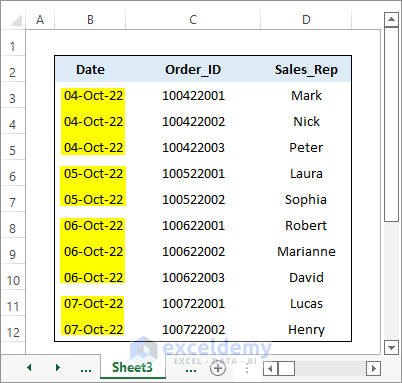
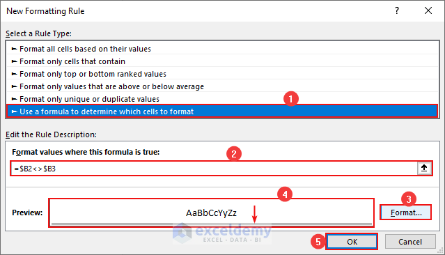
- First, select the range and go to Home >> Conditional Formatting >> New Rule. Then select Use a formula to determine which cells to format as the rule type. After that, enter the following formula in the formula box.
=$B2<>$B3- Next, click on Format, select the Bottom Border from the Border tab and click OK.
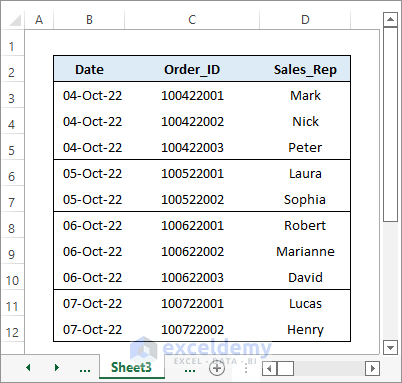
- After that, you will see the following result.
- You can use the following formula instead to group columns based on their values.
=B$2<>C$2Read More: How to Copy Conditional Formatting to Another Workbook in Excel
4. Conditional Formatting with Borders for Dynamic Ranges
Assume you need to apply conditional formatting to apply outside borders to a dynamic range. Follow the steps below to be able to do that.
📌 Steps:
- First, consider an extended range to which you need to enter data (for example, B2:D50). Then select the leftmost column (B2:B50) within the range and go to Home >> Conditional Formatting >> New Rule.
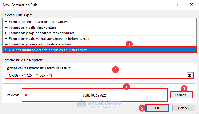
- Next, select Use a formula to determine which cells to format as the rule type. After that, enter the following formula in the formula box.
=OR(B2<>"",C2<>"",D2<>"")- Now click on Format, select the Left Border from the Border tab, and click OK.
- Then, apply a new conditional formatting rule on the same range using the following formula. But this time select the Left and Bottom borders in the Format Cells dialog box.
=AND(OR($B2<>"",$C2<>"",$D2<>""),$B3="",$C3="",$D3="")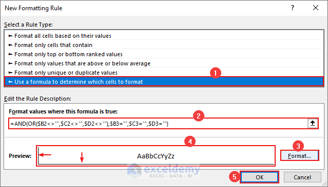
- Next, apply a new conditional formatting rule to the rightmost column (D2:D50) within the range using the following formula. Select the Right Border in the Format Cells dialog box in this case.
=OR(B2<>"",C2<>"",D2<>"")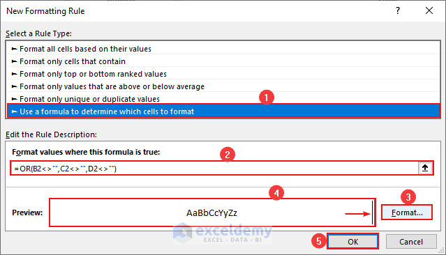
- Then, apply another new conditional formatting rule on the same range using the following formula. But this time select the Right and Bottom borders in the Format Cells dialog box.
=AND(OR($B2<>"",$C2<>"",$D2<>""),$B3="",$C3="",$D3="")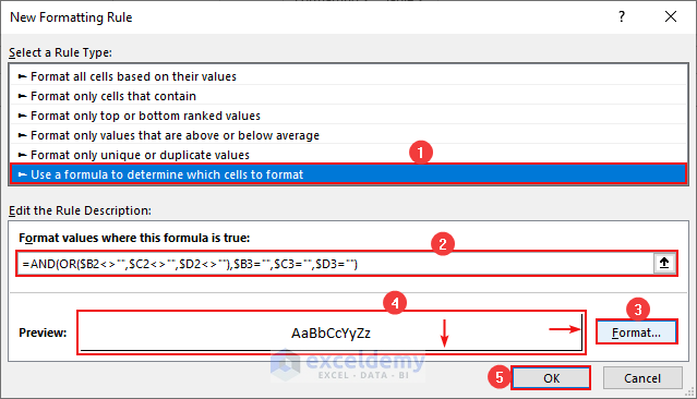
- Finally, select the middle columns (in this case, range C2:C50 only) and apply another conditional formatting rule using the following formula. You must select the Bottom Border only in this case.
=AND(OR($B2<>"",$C2<>"",$D2<>""),$B3="",$C3="",$D3="")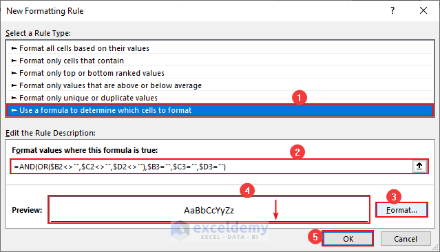
- Now enter values anywhere within the extended range (B2:D50) and the outline border will be extended automatically to include that data.
Read More: How to Copy Conditional Formatting But Change Reference Cell in Excel
Things to Remember
- You must select the desired range before creating a new conditional formatting rule.
- The formulas contain mixed references. Enter them properly otherwise, you won’t get the desired result.
Download Practice Workbook
You can download the practice workbook from the download button below.
Conclusion
Now you know how to apply conditional formatting borders in Excel. Do you have any further queries or suggestions? Please let us know in the comment section below. Stay with us and keep learning.
Related Articles
- How to Make Yes Green and No Red in Excel
- How to Create a Rating Scale in Excel
- How to Use Conditional Formatting on Text Box in Excel
- How to Apply Alignment in Excel Conditional Formatting
- How to Copy Conditional Formatting to Another Cell in Excel
- How to Copy Conditional Formatting Color to Another Cell in Excel
<< Go Back to Conditional Formatting | Learn Excel
Get FREE Advanced Excel Exercises with Solutions!
