Microsoft Excel is a great tool to create charts as it offers many predefined layouts and styles. We can even create our own customized style. In this article, we are going to learn how we can change chart style and set it to Style 8 which is one of the sixteen predefined styles that Excel provides. So let’s get started.
Change the Chart Style to Style 8: 2 Easy Methods
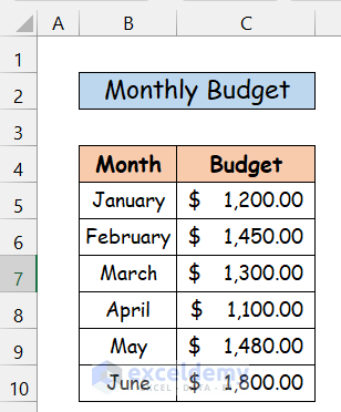
In this section, we will demonstrate 2 effective methods to change chart style to Style 8 in Excel with appropriate illustrations. But before that, first, let’s take an example where we have a data set. (see the figure below)
Based on this data, we have created a chart.
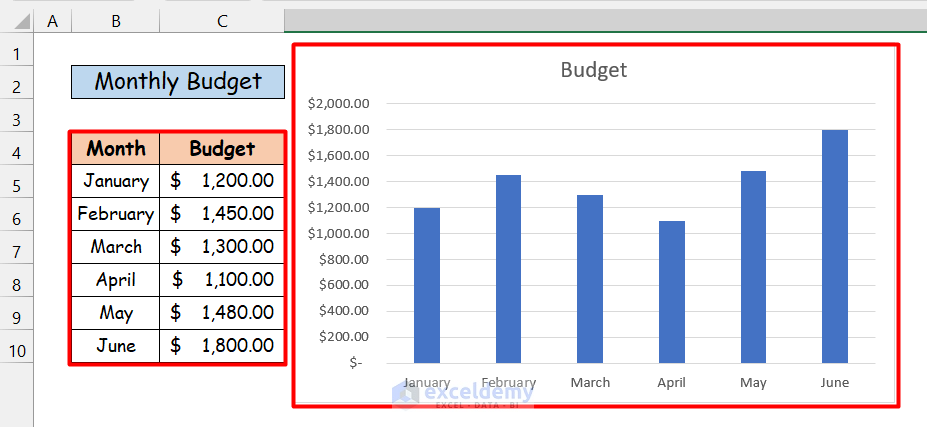
As we can see, this chart is in the default style, Style 1. On the other hand, there is a total of 16 predefined styles in Excel (Style 1, Style 2, and so on). and sometimes, we may need to change the style of the chart to suit our needs and preferences. For example, maybe we want to change the style of the chart to style 8. Here I have listed 2 methods to change chart style to Style 8.
1. Use of Chart Design Tab to Change Chart Style
In the first method, we will use the Chart Design Tab to change the chart style. To do that, follow the steps below.
Steps:
- First, click on any part of the chart. As soon as you click on the chart, you should see a new tab has appeared on the ribbon.
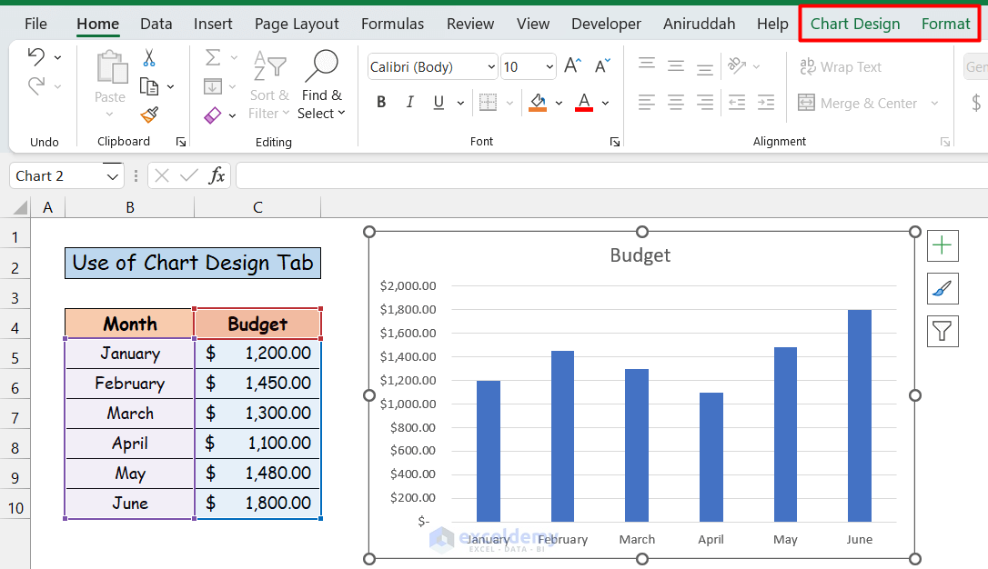
- Now, click on the Chart Design You should see many options like the figure below.
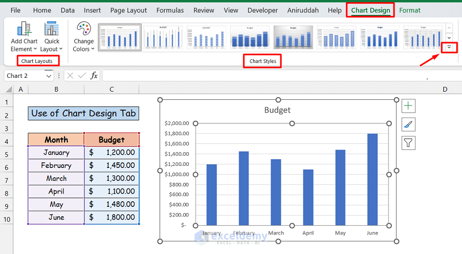
- Then, click on the arrow sign (▾) marked by the red rectangle box in the figure above. You should see all the predefined chart styles appearing.
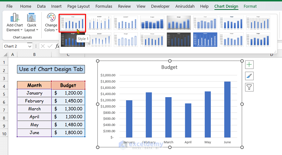
- Here, we can see that the current style is Style 1.
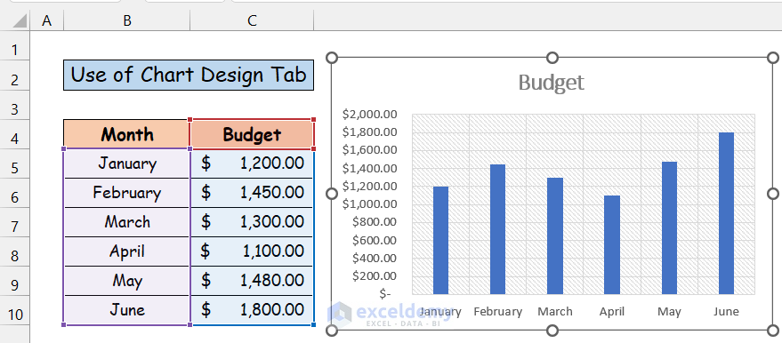
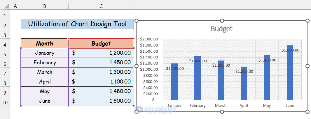
- Subsequently, if we select style 8, we will get the result shown below.
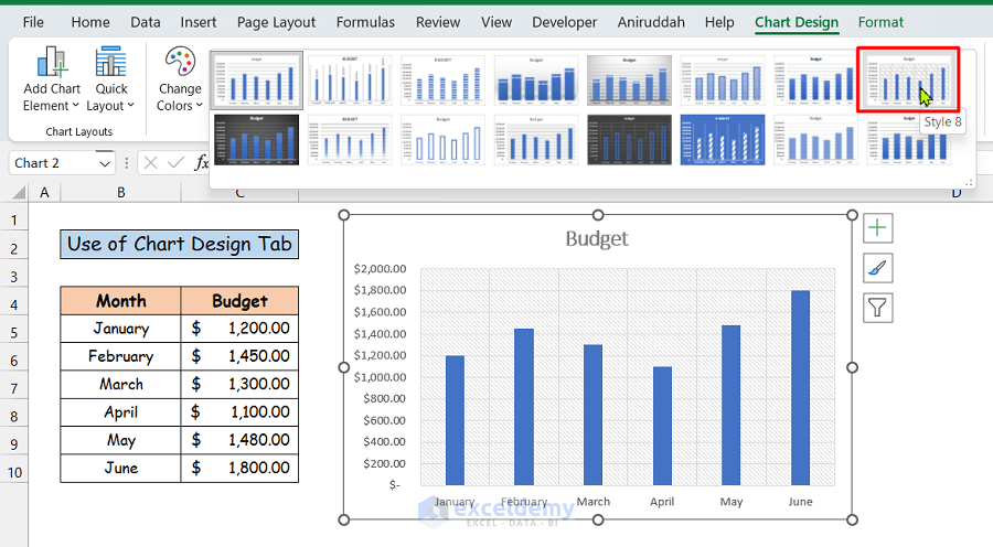
- Hence, our desired Style 8 chart will be like this.
2. Changing Chart Style with Chart Styles Tool
There is another alternative way which is quicker than using the Chart Design tab. Here we will use one of the tools that are adjacent to charts. To do that, follow the steps below.
Steps:
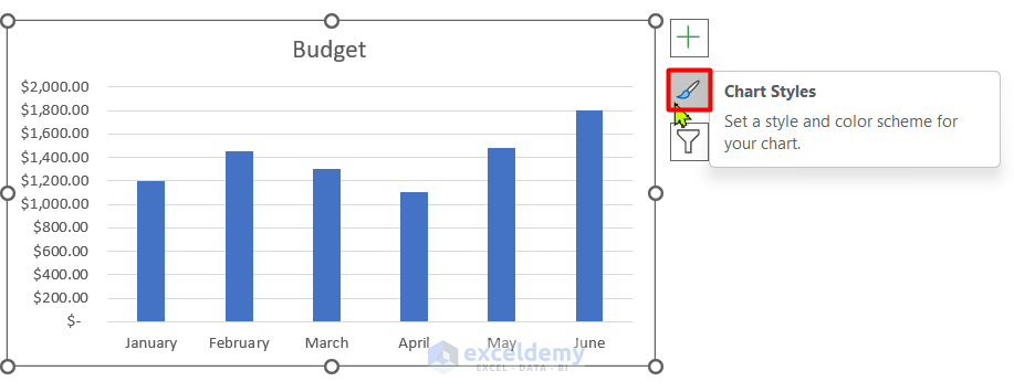
- First, click on the chart. You will see a toolbox containing 3 tools just on the right side of the chart.
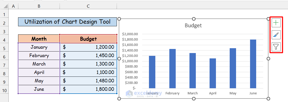
- The 3 tools that we can see are Chart Elements, Chart Styles, and Chart Filters respectively from top to bottom. They are very handy tools to customize the chart.
- Then, we will click on the Chart Styles option.
- Consequently, you will see many style options similar to what we have seen in method 1. As we want to select Style 8, scroll down below.
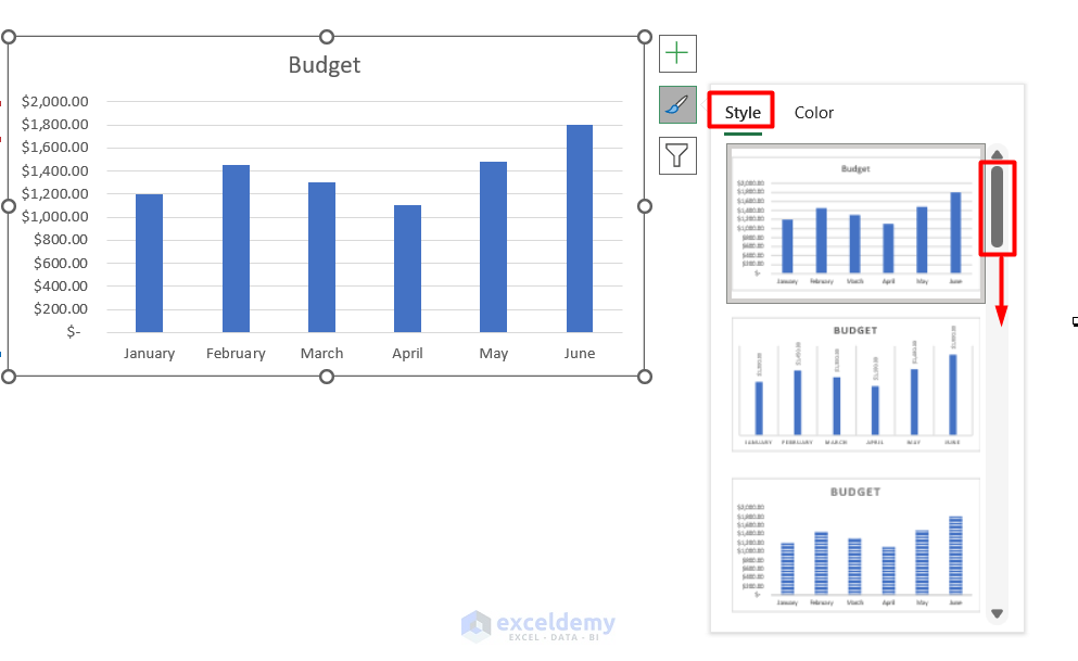
- As we hover the mouse cursor around styles, we will see a preview of the style on our chart. Now, select the Style 8.
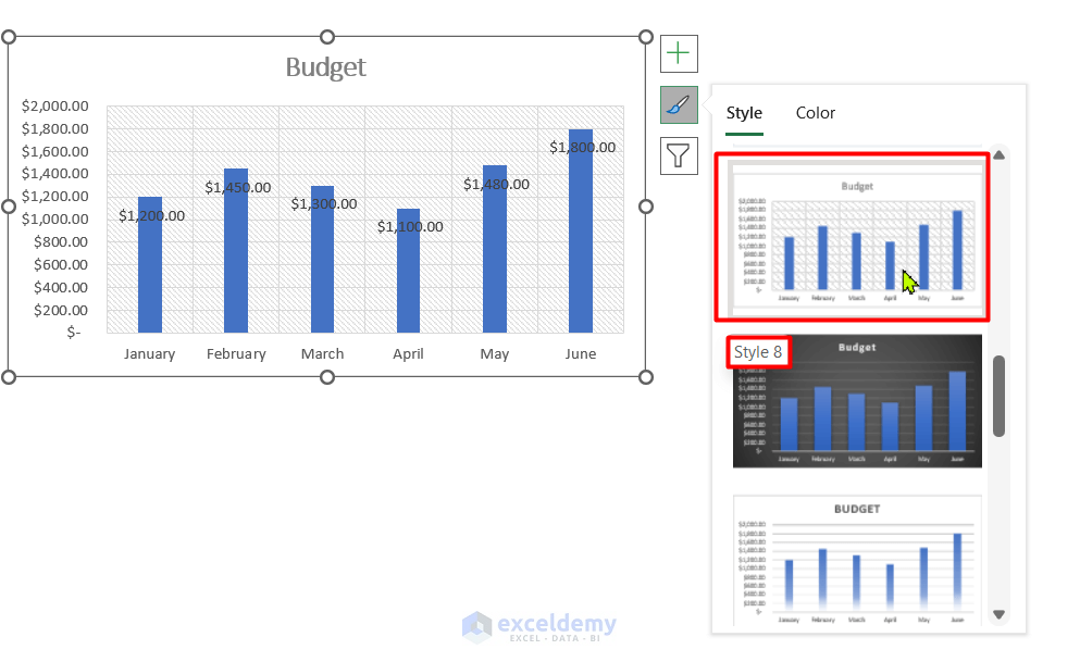
- As a result, you get your chart in Style 8
Things to Remember
- We can change the layout as well by using the 1st method.
- We also have the option to change the color of the style.
Download Practice Workbook
Download this practice workbook to exercise while you are reading this article.
Conclusion
That is the end of this article. Hopefully, you have a fair idea of how we can change the chart style to style 8. If you find this article helpful, please share this with your friends. Moreover, do let us know if you have any further queries.
Related Articles
<< Go Back to Chart Style in Excel | Excel Charts | Learn Excel
Get FREE Advanced Excel Exercises with Solutions!
