In our daily calculation and management work, we need to evaluate the Sales Margin of different products and services. If you are curious to know how you can calculate the Sales Margin in Excel, this article may come in handy for you. In this article, we are going to show how you can calculate the Sales Margin in Excel with elaborate explanations.
Overview of Sales Margin
Definition
The Sales Margin, also known as the contribution margin is the percentage of people make from selling product or service, with respect to the revenue. Usually calcularted in per unit account.
General Formula

How to Calculate Sales Margin in Excel: Step-by-Step Procedure
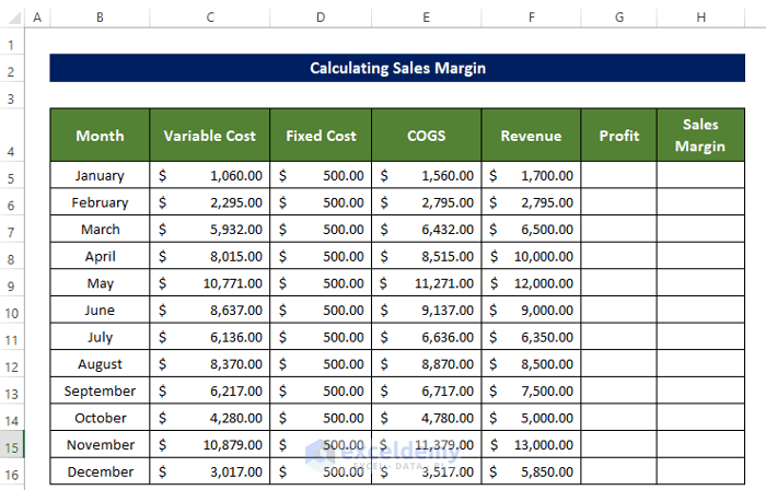
For the demonstration purpose, we are going to use the below dataset. In this table, all the costs related to the calculation of the Sales Margin like the Fixed Cost, Variable Cost, and Revenue are presented.
Step 1: Prepare Dataset
First and foremost, we need to prepare our dataset properly to prevent any kind of unwarranted and corrupted results.
We need to first prepare a separate table for the calculator of Variable Cost and Fixed Costs. After then we can calculate the sales margin.
Step 2: Calculate Profit
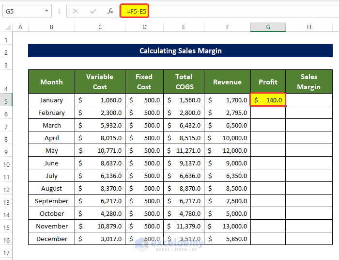
Right after we prepare the dataset, we will calculate the Profit.
- In the beginning, select the cell G5 and enter the following formula:
=F5-E5
Doing this will show the Profit for the month of January (cell B5) in cell G5.
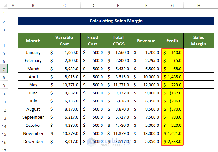
- After that, drag the Fill Handle from the corner of cell G5 to the corner of cell G16.
Doing this will fill the range of cells G5:G16 with the Profit value for each month in the range of cells B5:B16.
Step 3: Calculate Sales Margin
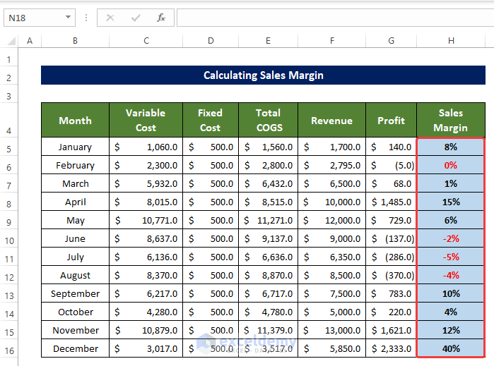
Finally, we will calculate the Sales Margin using the Profit calculated in the previous step.
- Select cell H5 and enter the following formula:
=G5/F5
- Doing this will show the Sales Margin for the month of January in cell H5.

- After that, drag the Fill Handle from the corner of cell H5 to the corner of cell H16.
- Doing this will fill the range of cells H5:H16 with the Sales Margin value for each month in the range of cells B5:B16.
💬 Note
Here, you can see some sales margin in a negative sign. This means there were no profits actually. It basically indicates the losses. On the other hand, if there is a positive sales margin, then the font will change back to black.
How to Calculate Gross Margin in Excel
In this method, we will discuss how we can determine the Gross Margin in Excel. We also used the SUM function in this method.
General Formula

Now, follow these steps to calculate gross margin using the above formula.
Step 1: Prepare Dataset
First and foremost, we need to prepare our dataset properly to prevent any kind of unwarranted and corrupted results. We need to first prepare a separate table for the calculator of Variable Cost and Fixed Costs. After then we can calculate the Gross Profit margin.
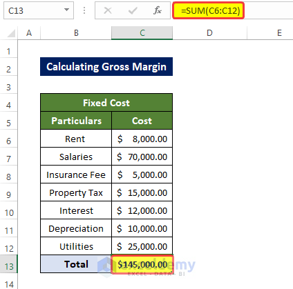
Step 2: Calculate Total Fixed Cost
After preparing the Dataset, we jump straight into calculating the Total Fixed Cost.
- Then we will select the cell C13 and enter the following formula:
=SUM(C6:C11)
- Doing this will calculate the sum of the Fixed Cost mentioned in the range of cells C6:C13.
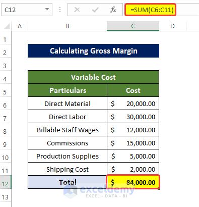
Step 3: Calculate Total Variable Cost
After calculating the Fixed Cost, the Total Variable Cost will be determined.
- We will select the cell C12 and enter the following formula:
=SUM(C6:C11)
- Doing this will calculate the sum of the Variable Cost mentioned in the range of cells C6:C11.
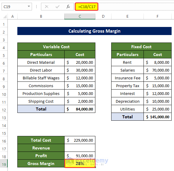
Step 4: Calculate Total Cost
We now calculate the Total Cost from the Variable Cost and Fixed Cost calculated in earlier steps.
- We will select the cell C16 and enter the following formula:
=SUM(C12,F13)
Cell C16 will now have the Total Cost from the summation of Variable Cost and the Fixed Cost.

Step 5: Calculate Profit
We now calculate the Profit from the Total Cost in cell C16 and the Revenue in cell C17.
- Select the cell C18 and enter the formula:
=C17-C16
Now we can see the Profit value in cell C18.

Step 6: Calculate Gross Margin
In this final step, we are going to evaluate the Gross Margin in cell C19.
- Select the cell C19 and enter the formula:
=C18/C17
Now we can see the Gross Margin value in cell C18.
How to Use Reverse Gross Margin Formula in Excel
We will determine how we can extract Revenue and Profit from the Gross Margin in Excel.
Step 1: Prepare Dataset
First and foremost, to prevent any unwarranted results and for the sake of clarity, we need to prepare the dataset properly.
- At first, you need to have all the necessary information related to the calculation of the revenue from the Gross margin
- In the dataset shown below, we have the Variable Cost, and Fixed Cost listed for each month.
- We also set the Gross Margin that we need to achieve with the given Total Costs.
- Now we need to estimate the revenue that we need to generate in order to meet the Gross Margin requirement mentioned in the range of cells F5:F16.
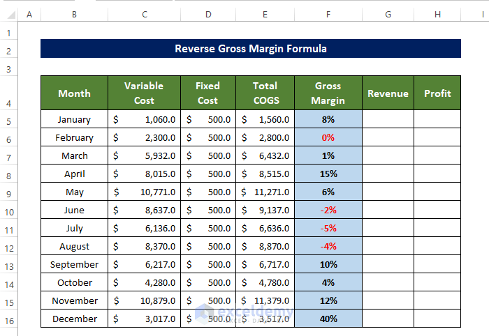
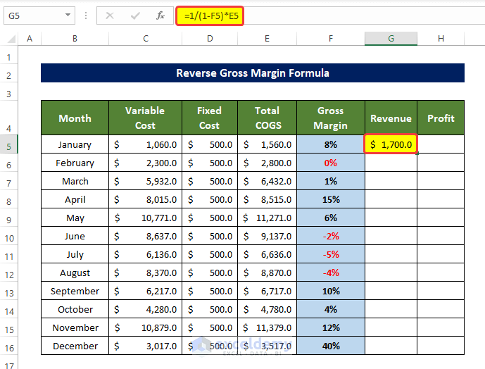
Step 2: Calculate Revenue from Gross Margin
Right after we prepare the dataset, we will calculate the Revenue.
- Select the cell G5 and enter the following formula:
=1/(1-F5)*E5
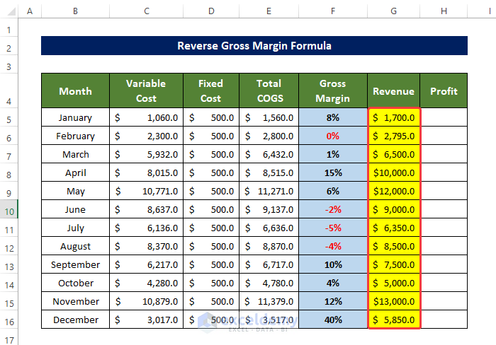
- After that, drag the Fill Handle from the corner of cell G5 to the corner of cell G16.
Doing this will fill the range of cells G5:G16 with the Revenue value for each month in the range of cells B5:B16. Which we need to generate to meet the Gross Margin requirement mentioned in the range of cells F5:F16.
Step 3: Calculate Profit
Furthermore, we will calculate the Profit after getting the Revenue value in the previous step.
- Select the cell G5 and enter the following formula:
=G5-E5
- Doing this will calculate the Profit for the month of January.

- After that, drag the Fill Handle from the corner of cell H5 to the corner of cell H16.
- Doing this will fill the range of cells H5:H16 with the Profit value for each month in the range of cells B5:B16. Which will be generated to meet the Gross Margin requirement mentioned in the range of cells F5:F16.

Download Practice Workbook
Download this practice workbook below.
Conclusion
To sum it up, the question “how to calculate Sales Margin in Excel” is answered here in 3 separate steps with elaborate explanations. Additionally, at the same time, we also estimated the Gross Margin and the Revenue from the Gross Margin via the reverse Gross Margin method.
For this problem, a workbook is available for download where you can practice these methods.
Feel free to ask any questions or feedback through the comment section. Any suggestion for the betterment of the Exceldemy community will be highly appreciated
<< Go Back to Margin | Formula List | Learn Excel
Get FREE Advanced Excel Exercises with Solutions!
