If you want to calculate negative margin in Excel, this article is for you. Here, we will walk you through 4 easy and effective methods to do the task effortlessly.
What Is a Negative Profit Margin?
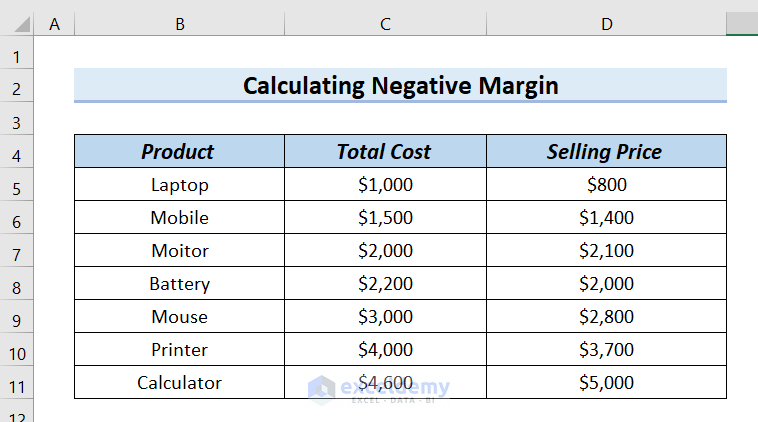
When the total cost for any quantity exceeds the selling price, it is called Negative Margin. In business terms, a Negative Margin indicates expending a larger amount of money than earning income.
How to Calculate Negative Margin in Excel: 4 Methods
The following table has the Product, Total Cost, and Selling Price columns. We will calculate the negative margin of this table using 4 different methods. Here, we used Excel 365. You can use any available Excel version.
1. Using Generic Formula to Calculate Negative Margin in Excel
In this method, we will use a generic formula to calculate negative margin in Excel.
Steps:
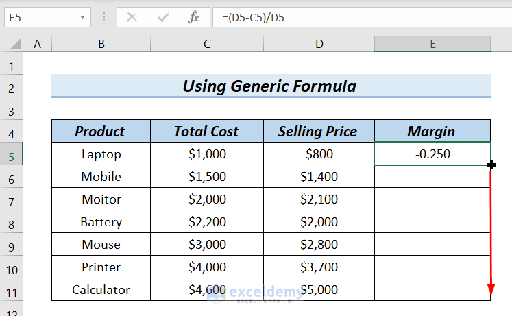
- First, we will type the following formula in cell E5.
=(D5-C5)/D5Here, the formula simply divides the value of D5-C5 by D5.

- After that, press ENTER. Then we will see the result in cell E5.
- Afterward, we will drag down the formula with the Fill Handle tool.
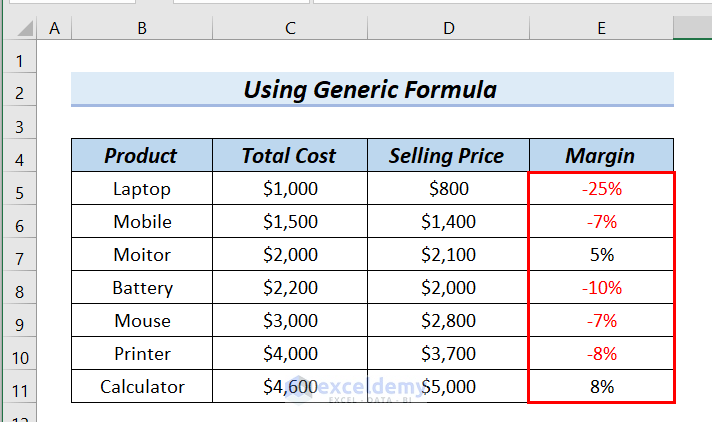
Now, we can see the complete Margin column. Here, we will highlight the negative margin value with Red color.

Now, we will add the Percentage to the Margin value.
- After that, we will select the entire Margin column >> go to the Home tab >> click on Percent Style (%).
You can also add the Percentage by selecting the Margin column and pressing CTRL+SHIFT+%.

Finally, in the Margin column, we can see calculate negative margin in Excel.
2. Use of IF Function to Calculate Negative Margin in Excel
Here, we will use the IF Function to calculate the negative margin in Excel. Here, we will use the IF function to avoid #DIV/0! error that may occur when the Selling Price is 0.
Let me show you the error first.
- To begin with, write the following formula in cell E5.
=(D5-C5)/D5- After that, we will press ENTER.

Here, you can see the output in cell E5 shows an error.
This is because cell D5 has a $0 Selling Price, and therefore, the denominator of the formula becomes 0. As a result, the error appears.
To get rid of this error now will use the IF function.
Steps:
- First, we will type the following formula in cell E5.
=IF(D5<>0,(D5-C5)/D5,0)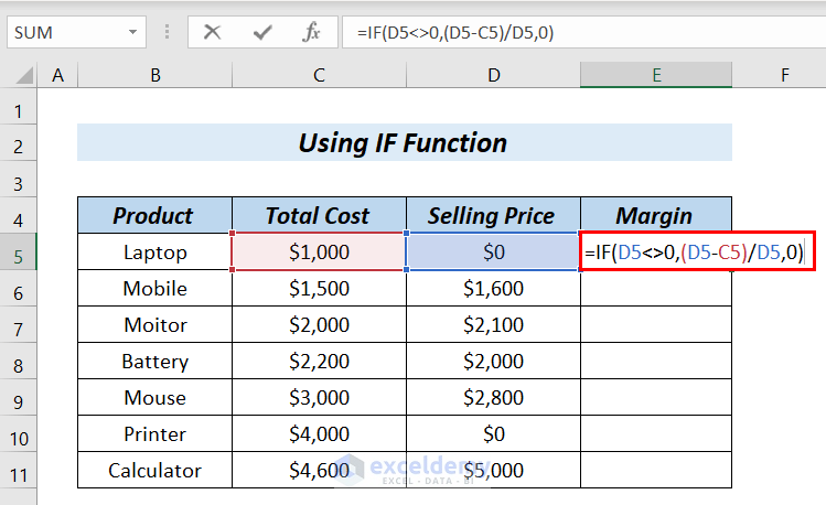
Formula Breakdown
- (D5-C5)/D5 → returns the value after dividing D5-C5 by D5.
- Output: #DIV/0!
- IF(D5<>0,(D5-C5)/D5,0) → The IF function returns value_if_true if the conditions is TRUE otherwise it returns value_if_false.
- IF(FALSE,#DIV/0!,0) → becomes
- Output: 0
- Explanation: As the condition is FALSE it returns the value of value_if_false.
- After that, press ENTER. Then we will see the result in cell E5.
- Afterward, we will drag down the formula with the Fill Handle tool.

- Next, we will highlight the negative margin value in Red color.

- After that, By following Method_1 steps, we will add the Percentage in the Margin column.
- Next, we Highlighted the Negative Margin with Red color.
Finally, we can see in the Margin column we can see calculate negative margin in Excel.

3. Applying IFERROR Function
In this method, we will use the IFERROR function to calculate negative margin in Excel.
Steps:
- First, we will type the following formula in cell E5.
=IFERROR((D5-C5)/D5,0)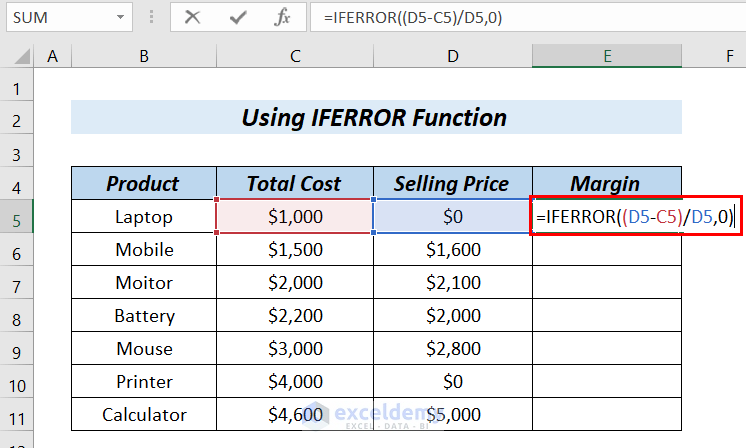
Formula Breakdown
- (D5-C5)/D5 → First, it will Subtract the Selling Price from the Total Cost then it will Divide it by the Selling Price.
- Output: #DIV/0!
- IFERROR((D5-C5)/D5,0) → The IFERROR function returns a given specific value for any error.
- IFERROR(#DIV/0!,0) → becomes
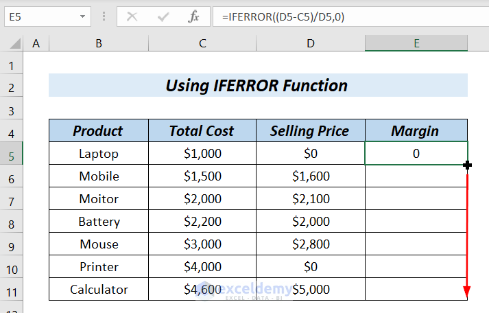
- Output: 0
- Explanation: Here, the IFFERROR function returns 0 as it founds an error.
- Afterward, press ENTER. Then we will see the result in cell E5.
- Then, we will drag down the formula with the Fill Handle tool.
- After that, By following Method_1 steps, we will add the Percentage in the Margin column.
- Next, we will highlight the negative margin value in Red color.
Finally, we can see in the Margin column we can see calculate negative margin in Excel.

4. Inserting Table to Calculate Negative Profit Margin
In this method, we will calculate negative profit margin in Excel. First, we will calculate the Profit, and after that, we will calculate Margin. To make the task easier, we will insert a Table before calculation.

Steps:
- First, we will select the Entire dataset >> go to the Insert tab >> select Table.

A Create Table window will appear.
Make sure My table has headers is marked.
- Then, click OK.

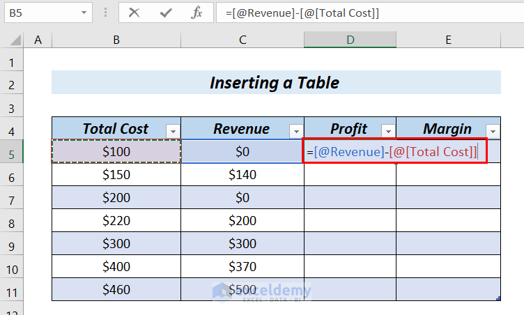
Next, we will see the inserted table.
- After that, we will type the following formula in cell D5 to calculate Profit.
=[@Revenue]-[@[Total Cost]]This formula simply subtracts Total Cost from Revenue.
- After that, press ENTER. We will see the complete Profit column.
Now, we will calculate Margin.
- Afterward, we will type the following formula in cell E5.
=IFERROR([@Profit]/[@Revenue],0)
Formula Breakdown
- [@Profit]/[@Revenue] → First, it will Divide the Profit by the Revenue.
- Output: #DIV/0!
- IFERROR([@Profit]/[@Revenue],0) → The IFERROR function returns a given specific value for any error.
- IFERROR(#DIV/0!,0) → becomes
- Output: 0
- Explanation: Here, the IFFERROR function returns 0 as it founds an error.
- After that, press ENTER.
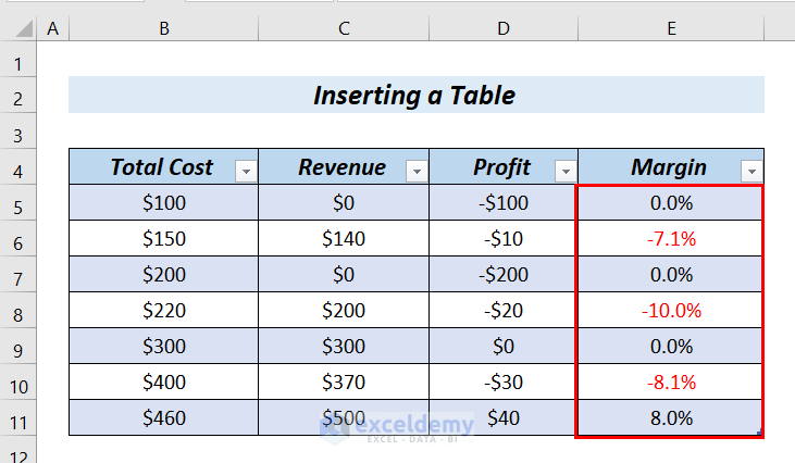
- After that, By following Method_1 steps, we will add the Percentage in the Margin column.
- Next, we will highlight the negative margin value in Red color.
Finally, in the Margin column, we can see the calculated negative profit margin in Excel.
Practice Section
In the practice section of your sheet, you can practice the explained methods.

Download Practice Workbook
Conclusion
Here, we tried to show you 4 methods to calculate negative margin in Excel. Thank you for reading this article, we hope this was helpful. If you have any queries or suggestions, please let us know in the comment section below. Please visit our website Exceldemy to explore more.
<< Go Back to Margin | Formula List | Learn Excel
Get FREE Advanced Excel Exercises with Solutions!
