Bank Interest Calculator in Excel Sheet – Download Free Template

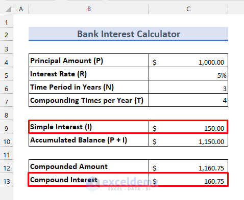
Here’s an overview of the bank interest calculator we will make.

Terms Related to the Bank Interest Calculation

Principal Amount (P): The balance at the beginning of the calculation.

Interest Rate (R): The rate at which interest is given.

Period (N): Number of periodic durations of the deposit or loan.

Compound Interest: Compound Interest extends to the added interests also. Banks mainly deal with compound interest.

Simple Interest: Simple interest works on the Principal Balance only. Banks may offer simple interest in special circumstances.

Compound Frequency (T): In the case of compound interest, interest is usually compounded daily, monthly, quarterly, semi-annually, and annually. Then the number of Compounding Times will be 365, 12, 4, 2, and 1 respectively.

Simple Interest Calculation in Excel

We can easily calculate Simple Interest using the following formula:

Steps

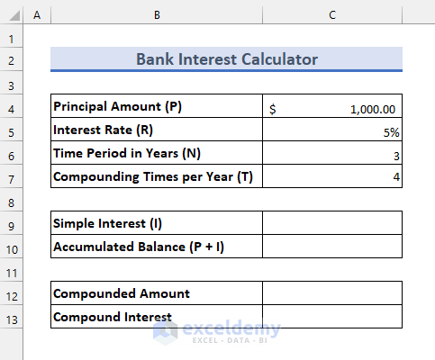
• We have the following dataset.

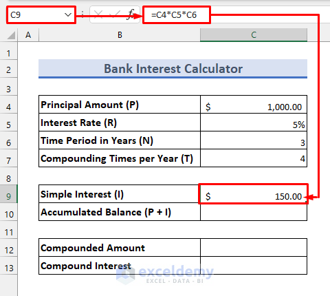
• To find Simple Interest, enter the following formula in cell C9:

• You will see the result as follows:

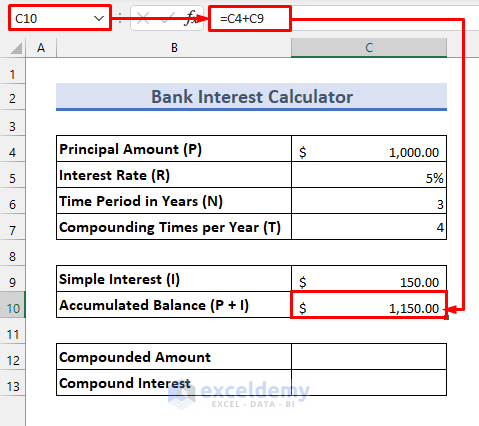
• To calculate the final balance with interest added, apply the following formula in cell C10:

• You will see the accumulated balance as shown below.

• At the end of each year, your account balance will be as follows.

Read More: Create a Daily Loan Interest Calculator in Excel

Compound Interest Calculation in Excel

We can calculate compound interest using the formulas given below.

• Compounded Amount (A) = P ✕ (1 +  I / T)  ✕ N ✕ T
• Compound Interest = (A – P)

Steps

• Apply the following formula in cell C12:

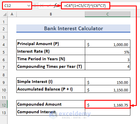
• Enter the following formula in cell C13 to get the compound interest.

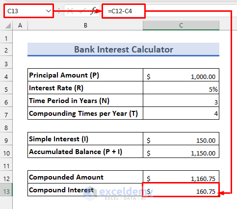
• At the end of each quarterly period, your account balance will be as follows.

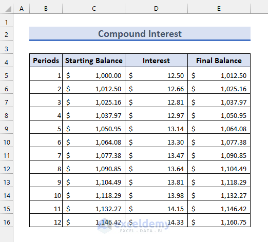
• You can use this as a template for your bank interest calculator Excel sheet.

Read More: How to Create a Daily Compound Interest Calculator

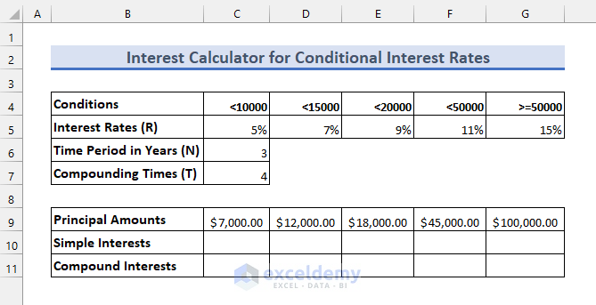
Bank Interest Calculation in Excel for Different Interest Rates

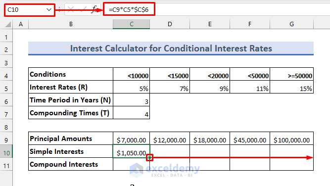
Assume that you need to calculate the interest rates for the following dataset.

Steps

• Enter the following formula in cell C10:

• Use the Fill Handle tool to get other interest amounts to the right.

• Apply the following formula in cell C11 to get the compound interest. Use the Fill Handle tool to apply for other cells in the row.

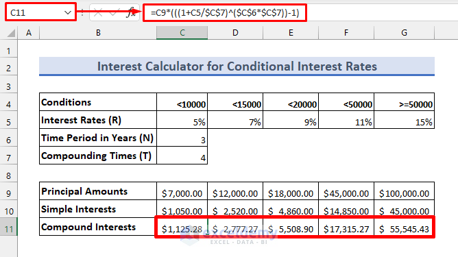
• Next, to understand the above formula, just compare it to the following formula:

• If you need to calculate the accumulated amounts, you can follow the methods above.

EMI Calculation Using the PMT Function in Excel

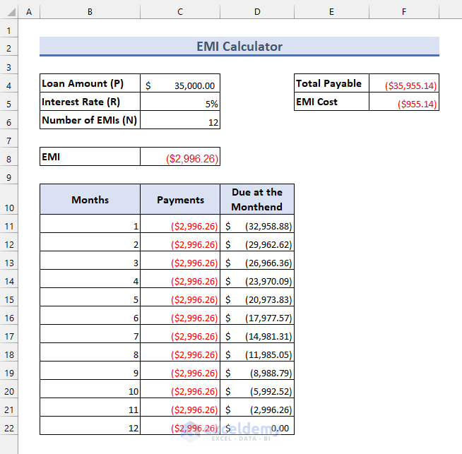
We want to buy a car for $35,000 and complete the payment in 12 EMIs at a 5% yearly interest rate. Let’s calculate the EMI.

Steps

• Apply the following formula in cell C8:

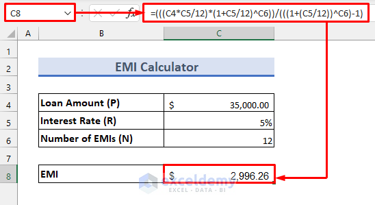
• Compare the result with the following formula.

Excel also has an inbuilt function called the PMT function to calculate EMI.

How does the formula work?

The PMT function has the following arguments:

• Rate = Rate of interest applied on the borrowing.
• NPER = Number of monthly installments per loan term which is N in this case.
• PV = Present value or Principal amount (P)
• FV = Future value after last payment which is 0 in this case
• Type = 1 or 0. The payment due at the beginning of the month indicates 1 and 0 if it is at the end of the month.

Here’s how to use it:

• Enter the following formula instead in cell C8:

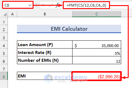
• Your monthly installments will be as follows.

Things to Remember

• Convert the yearly interest rate to monthly, quarterly, etc. interest rate by dividing it by the compounding times (T).
• Make sure to use the absolute references properly.

Download the Bank Interest Calculator

Further Readings

• Create Reverse Compound Interest Calculator in Excel
• Make Quarterly Compound Interest Calculator in Excel
• How to Develop CD Interest Calculator in Excel
• How to Create SIP Interest Calculator in Excel
• How to Generate Overdraft Interest Calculator in Excel

<< Go Back to Finance Template | Excel Templates