Latest Posts From Zahid Hasan

Method 1 - Find y Intercept to Calculate Standard Deviation in Excel Find the y-intercept of the given dataset. We can use various functions to find the ...

The sample dataset showcases the Marks of Grade 6 Students. After opening the Excel file, a warning is displayed: Solution 1 - Using the Document ...
Method 1 - Using Text Box Command from Insert Tab Steps: Go to the Insert tab from Ribbon. Choose the Text Box option from the Text group. ...

We frequently need to carry out some challenging mathematical computations while using Excel. The majority of these intricate mathematical calculations can be ...

We have the Store Location of different cars in different stores. The Serial Number follows a RegEx pattern but there are some cars that have the same Serial ...

In Excel, we often need to do various types of mathematical calculations. Anchoring columns is a common practice when performing these calculations. In this ...

While working in Excel, we often need to filter a large dataset based on specific tags. Filtering datasets in this manner can save a significant amount of time ...
Our dataset includes the Addresses of ABC Company employees. Our goal is to find the ZIP Codes from the given addresses. Method 1 - Applying Excel ...

The Sales Data of XYZ Store is the sample dataset. Create a Sunburst Chart and rotate it. Method 1 - Using the Camera Tool Steps: ...
Method 1 - Counting Cells Greater Than 1 in a Single Column We have the Sales Status of a Store as our dataset. We'll find the number of Items that ...

What Is a Contingency Table? Contingency Tables are a summary of various categorical variables. Contingency Tables are also known as Cross Tabs and Two-way ...

Suppose you have the following data set: Example 1 - Counting Cells While Excluding Some Specified Cells Steps: Choose an appropriate cell, ...
Method 1 - Using COUNTIF Function to Calculate Frequency in Excel Steps: Use the following formula in cell D17. =COUNTIF($C$5:$C$14,"<="&B17) ...
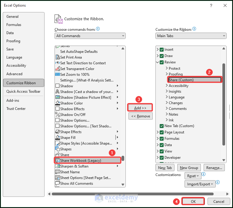
The dataset showcases the Sales Analysis of the XYZ Store. If you go to the Review tab on the Ribbon, you will see that the Unshare Workbook option is ...

Method 1 - Unprotecting Worksheet Step 01: Pasting Link in a Protected Worksheet See what happens when we try to paste a link into a protected worksheet. ...
- « Previous Page
- 1
- 2
- 3
- 4
- …
- 6
- Next Page »
See Our Reviews at


I am sorry to hear that. Could you maybe describe which step of the procedure you are having trouble with so that I can clear up any confusions? Both methods worked fine for me. I have got the following output using these methods.
Dear AL,
Thank you for your query. So, your goal is to import data from a CSV file that has a column named ID with 20 digits in each cell of the column. You can use the following procedure to avoid converting the data into scientific notation while importing the CSV file.
First, create a CSV file with the required data. For demonstration, I have used the following data.
Now, go to the Data tab >> click on From Text/CSV.
Then navigate to your file and select it >> click on Import.
Next, click on the drop-down button >> choose the Do not detect data types option >> click on Load.
That’s it! Your data has been successfully loaded into Excel without any conversion to scientific notation or data loss.
I believe this has addressed your query. If you require additional support, please don’t hesitate to inform us.
Regards
Zahid
ExcelDemy
Hello ROBYRUBYJANE,
Thank you for your query. To create a search box that will search data based on a provided date, you can follow the steps given below.
First, construct a search box and add this code to it.
In this code, “Sheet9” refers to the specific worksheet containing the data that requires searching based on dates. The code we have used employs the “greater than or equal” operator, indicating that any data with dates preceding the specified date will not appear in the output.
I hope this answers your question. If you have any more queries, please please reach out to us.
Regards
Zahid
ExcelDemy
Hello ROBYRUBYJANE,
Thank you for reaching out. If I understand correctly, you are interested in creating a search box that can locate values from another worksheet and transfer them to the current worksheet. To accomplish this, you can use the following steps:
Begin by creating a search box, and then add the following code to it.
In this scenario, “Sheet4” is the worksheet containing the search box, and any copied values will be pasted into the range B6:D19 of this worksheet. Prior to pasting, the contents and formatting of the destination range will be cleared. “Sheet6” is the worksheet where the specified keyword will be searched for.
With these steps completed, your search box is now ready for use.
I hope this helps you to achieve your goal. If you need further assistance in this regard, please let us know.
Regards
Zahid
ExcelDemy
Hello AMIT,
I appreciate your question. I’d like to clarify that in this article, the expression “Current Volatility” refers specifically to Implied Volatility, rather than Realised Volatility. When working with Option Probability, it’s generally more advantageous to use Implied Volatility rather than Realised Volatility since it enables us to make more precise predictions about the projected price range of a stock in the future.
I hope this answers your question. If you have any more queries, please let us know.
Regards
Zahid
ExcelDemy
Dear UDAY KUMAR,
Good afternoon! Thank you for reaching out to us. In the following section, I’ve suggested a method for handling your issue.
First, apply this formula in cell M2.
=LAMBDA(item_name,max_issue,XLOOKUP(SEQUENCE(SUM(max_issue)),VSTACK(1,SCAN(1,max_issue,LAMBDA(a,b,a+b))),VSTACK(item_name,""),,-1))(H2:H5,I2:I5)Formula Breakdown
In this formula, item_name refers to the cell range H2:H5 of your provided worksheet, and max_issue represents the cell range I2:I5 of that worksheet.
XLOOKUP(SEQUENCE(SUM(max_issue)),VSTACK(1,SCAN(1,max_issue,LAMBDA(a,b,a+b))),VSTACK(item_name,””),,-1)) → This part of the formula will generate the Item Names according to their maximum issue number.
(H2:H5,I2:I5) → This part is required for specifying the cell ranges for item_name, and max_issue parameters of the formula.
After applying this formula, you will get an output like this in your worksheet.
Now, select these cells and copy them. Later, paste them as values in the same location.
Now, apply the following formula in adjacent cell N2 and drag the Fill Handle up to cell N32.
=RAND()After that, select the data of Column M and Column N. Then, go to the Sort & Filter option from the Home tab and choose the Custom Sort option from the drop-down.
A dialogue box named Sort will appear on your worksheet. In the Sort by field, select Column N. You can keep the other fields unchanged. Finally, click OK.
Lastly, select the entire Column N and delete it.
After following these steps, you will have a randomized list of Item Names for a month as demonstrated in the following image.
I sincerely hope that this resolves the issue that you are facing. If you need any further assistance, please let us know. Have a great day!
Regards
Zahid Hasan
ExcelDemy
Dear Mohtasham,
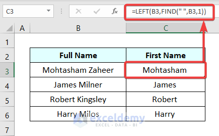
Thank you for your query. You wanted to extract a text value from a cell until a blank space appears in the text. It can be easily achieved by using a combination of LEFT function and FIND function in Excel. The formula is given below.
=LEFT(B3,FIND(” “,B3,1))
Here, we have our original text in cell B3. We applied this formula in cell C3.
The FIND function will return the position of the first space in the text of cell B3. Then, the LEFT function will extract the texts up to that position from the left side of the text. You can drag the Fill Handle to copy down the formula for other cells as well. The following image demonstrates the formula and its associated outputs.
I truly hope that this answers your question. Again thank you for reaching out to us. Please let us know in the comments area if there is anything about this approach that is unclear to you. I wish you all the best!
Regards
Zahid Hasan
ExcelDemy
Dear Uday Kumar,
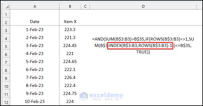
Good day! I can comprehend how upsetting this situation could be. It took me a while to understand it, too. Hence, the portion of your formula that I have highlighted in the following figure is essentially what is causing the issue when doing Conditional Formatting.
It will display an error in the Conditional Formatting when you specify a range using both a cell reference and a formula. As the goal of this formula is to add up to the cell that comes before the active cell, you can use the following formula instead. Here I simply replaced INDEX(B$3:B3,ROWS(B$3:B3)-1) by B2. The complete formula is:
=AND(SUM(B$3:B3)>B$35, IF(ROWS(B$3:B3)<>1, SUM(B2:B$3)<=B$35, TRUE))
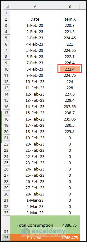
Just paste this formula in the Conditional Formatting option and you will have your desired output as shown below.
That should take care of your problem, I hope. If you run into any problems, please let us know.
Regards
Zahid Hasan
ExcelDemy
Good day, Don Rogers.
Thank you for your feedback. Could you please share your excel file with me so that I can better understand your problem and provide you with a solution? You can shareyour file to the email address provided below.
[email protected]
Thank you!
Dear Uday Kumar,
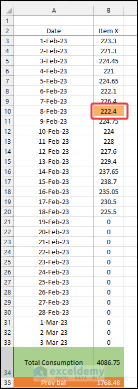
Good afternoon! First of all, thank you for the detailed description of the problem. What I have understood from your email, is that you want to highlight the cell where the sum of the distributed X items crosses the Previous Balance.
Using the Excel formula in this situation becomes quite complicated and returns errors when used in the Conditional Formatting option. But running a simple Macro can achieve your desired output without any hassle.
If you don’t know how to run a Macro, don’t worry. It’s not that complicated at all. Just follow the steps below, and you will be good to go.
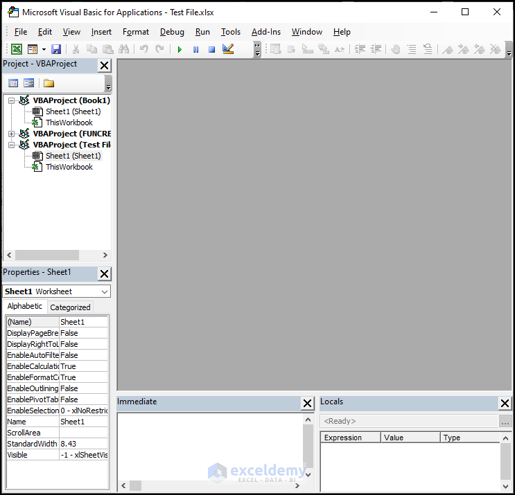
Step 01: Create a Blank Module
At first, you will need to create a blank Module. The Module is where we will write the code. Simply press ALT + F11 on your keyboard to open the following window on your worksheet.
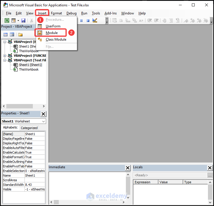
Now, go to the Insert tab and choose the Module option from the drop-down list.
Step 02: Write and Run VBA Code
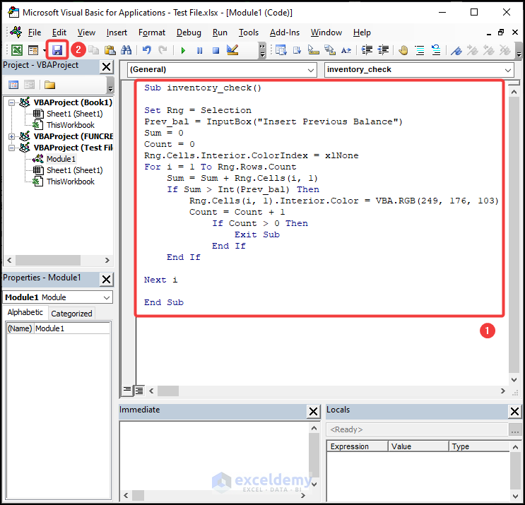
Now, a blank Module will be created.
Then, copy the following code and paste it into the blank Module.
After that, click on the Save icon.
Following that, close the VBA window or simply press ALT + F11. This will take you back to your worksheet.
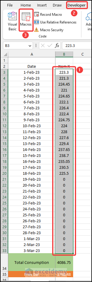
Now, carefully select the range of data.
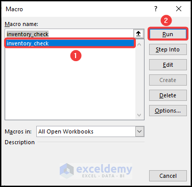
Then, go to the Developer tab and click on the Macros option.
Subsequently, the Macro dialogue box will open.
Now, select the inventory_check option and click on Run.
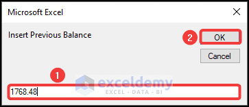
Then a window will appear asking you for the Previous Balance. You need to enter the previous balance here and then click OK.
Boom! The highlighted cell will indicate your desired output.
You can change the Previous Balance according to your need and the highlighted cell will be changed accordingly.
Things to Remember
If you don’t have the Developer option enabled then follow this article to enable it.
Don’t forget to save the file as Macro Enabled Workbook.
I sincerely hope that this solves the issue you are facing. If any part of the solution is unclear to you, please let us know.
Regards
Zahid Hasan
ExcelDemy