How to Copy Chart Without Source Data and Retain Formatting in Excel: 2 Simple Methods

Method 1 – Using Paste Special Option

Step 01: Create Chart for 1st Term

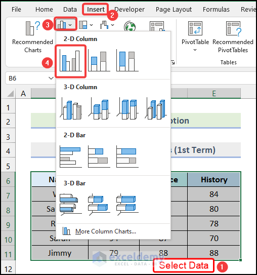
• Select the dataset and go to the Insert tab from Ribbon.
• Choose the Insert Column or Bar Chart option.
• Click on the Clustered Column option from the drop-down.

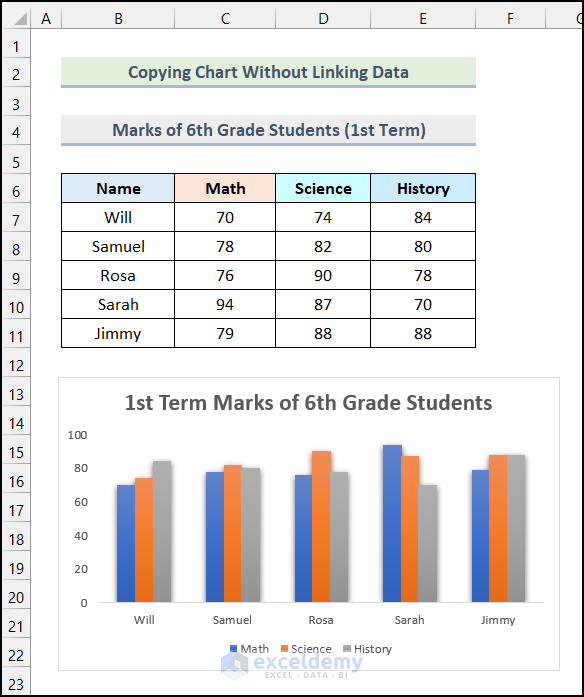
You will have the following chart on your worksheet.

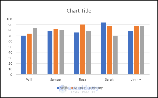
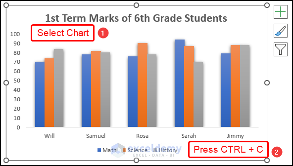
• You can modify and format the chart to get the following output.

Step 02: Create Chart for 2nd Term

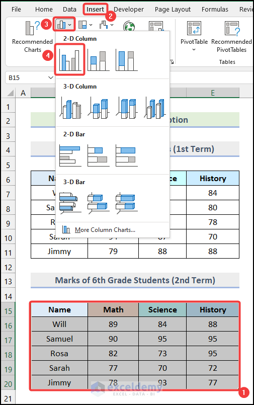
• Select the dataset for 2nd Term and go to the Insert tab from Ribbon.
• Click on the Insert Column or Bar Chart option
• Select the Clustered Column option from the drop-down.

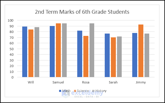
You will have the following chart in your worksheet as shown in the following image.

• Click on the chart for 1st Term and press the keyboard shortcut CTRL + C to copy the chart.

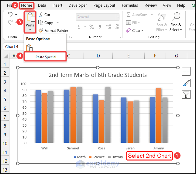
• Click on the chart for 2nd Term and go to the Home tab from Ribbon.
• Click on the Paste option from the Clipboard group.
• Select the Paste Special option from the drop-down.

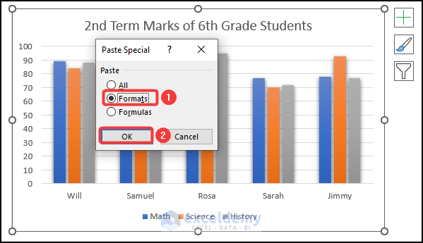
• Choose the Format option from the Paste Special dialogue box.
• Click OK.

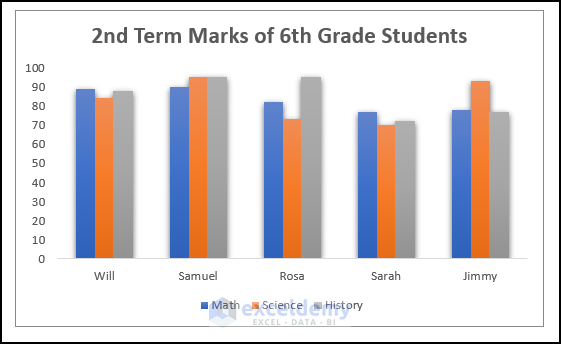
Yoy successfully copied a chart without source data and retained formatting in Excel. Your final output should look like the following picture.

Method 2 – Saving Chart as Template

Steps:

• Use the steps mentioned in Step 01 of the 1st Method to obtain the following output on your worksheet.

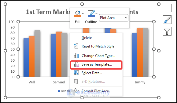
• Right-click on any portion of the chart area.
• Select the Save as Template option.

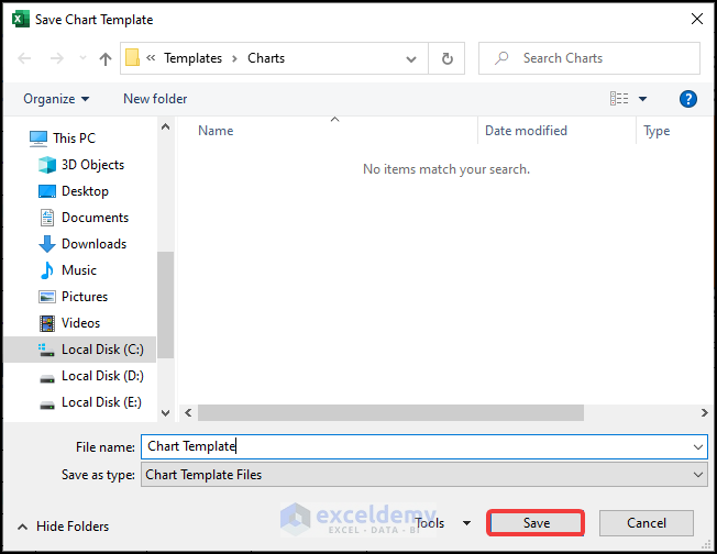
• Rename the template file according to your preference and click on Save. We used Chart Template as our file name.

Note: Don’t change the location while saving the file. Just use the default location that is suggested by Excel. If you change the location, you will not be able to see your template inside Excel.

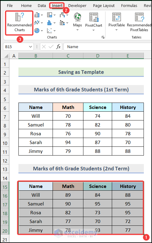
• Select the data for the 2nd Term and go to the Insert tab from Ribbon.
• Click on the Recommended Charts option from the Charts group.

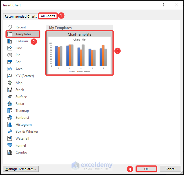
The Insert Chart dialogue box will open on your worksheet, as shown in the image below.

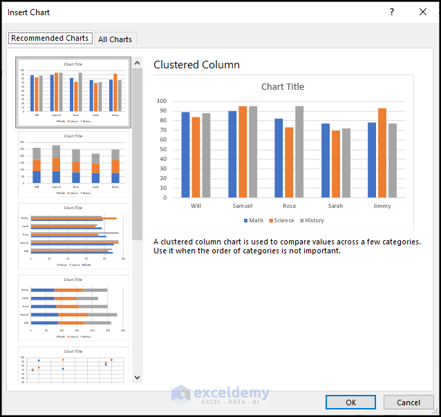
• Go to the All Charts tab in the Insert Chart dialogue box.
• Click on the Templates option.
• Select your created template as marked in the following picture.
• Click OK.

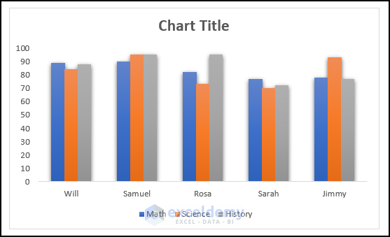
You will have the formatting of the chart of the 1st Term applied to the newly created chart.

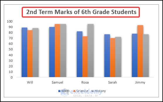
• Change the title of the chart. We used 2nd Term Marks of the 6th Grade Students as our chart title.

How to Copy Chart Without Linking Data in Excel

Steps:

• Use the steps mentioned in Step 01 of Method 1 to get the following output.

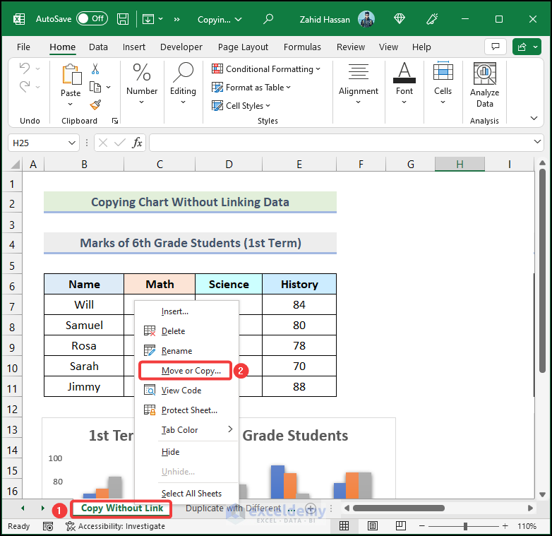
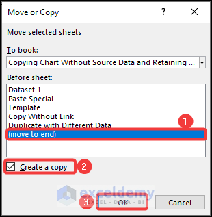
• Right-click on the worksheet name and choose the Move or Copy option.

• From the Move or Copy dialogue box, select the (move to end) option.
• Check the field of Create a copy.
• Click OK.

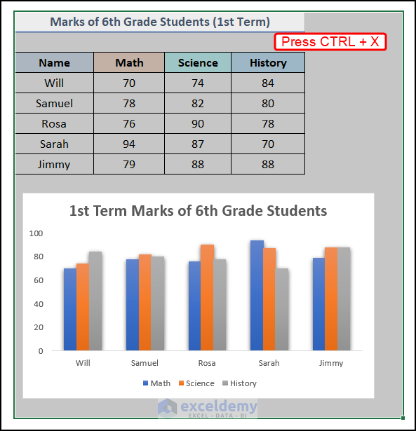
An identical worksheet will be created, as shown in the image given below.

• Select the dataset and the chart of the newly created worksheet.
• Press the keyboard shortcut CTRL + X.

• Go back to the original worksheet and press CTRL + V to paste the copied dataset and the chart.

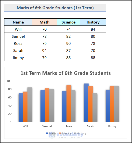
• Change the copied dataset as you want, and your chart will be changed accordingly.

We inserted the Marks of the 2nd Term, and the chart has adjusted automatically according to our change in the dataset.

How to Duplicate Chart with Different Data in Excel

Steps:

• Follow the procedure discussed in Step 01 of the 1st Method to obtain the following output.

• Click on the chart and use the keyboard shortcut CTRL + C to copy the chart.

• Select any cell of the worksheet and press CTRL + V to paste the copied chart.

• Right-click on any portion of the pasted chart and choose the Select Data option.

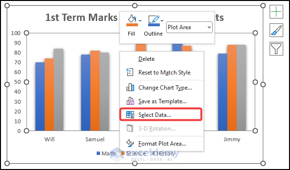
The Select Data Source dialogue box will open on your worksheet.

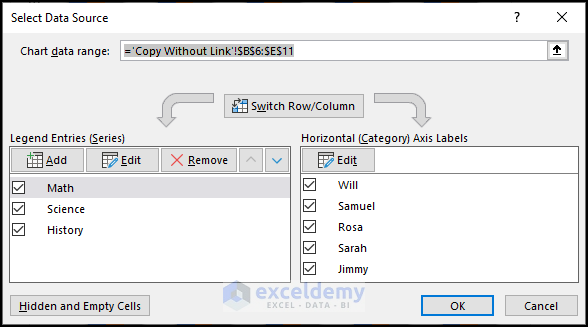
• Click the Chart data range field in the Select Data Source dialogue box.
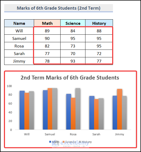
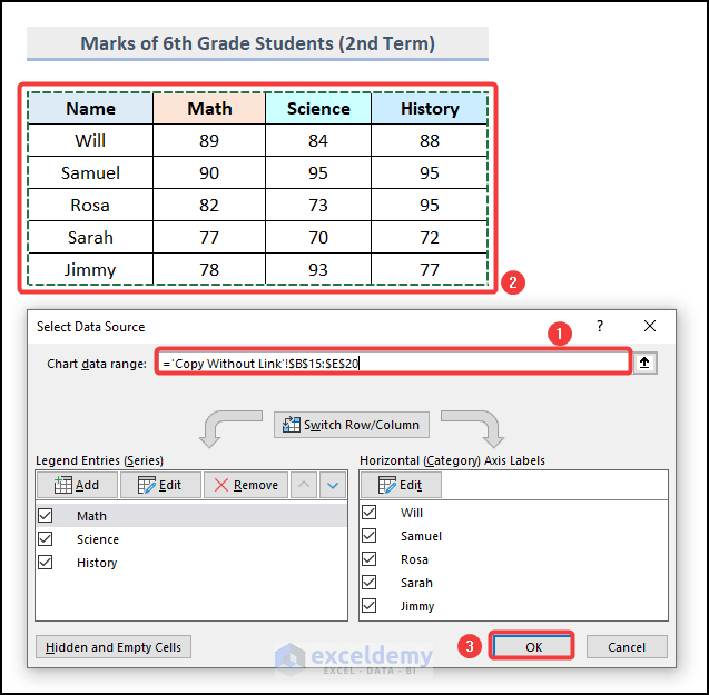
• Select the cells of the Marks of 6th Grade Students (2nd Term) table as the new chart data range.
• Click OK.

You have the following output as demonstrated in the following picture.

• Add a new chart title. We used 2nd Term Marks of 6th Grade Students as our new chart title.

Download Practice Workbook

<< Go Back To Copy Chart in Excel | Excel Charts | Learn Excel