Latest Posts From Md. Shamim Reza

The Bullets and Numbering feature is not usually available on the Ribbon. To enable it: Right-click the Home tab and select Customize the Ribbon. ...

This article illustrates how to make a t-distribution graph in Excel. Distribution in statistics deals with the relationships between observations and their ...
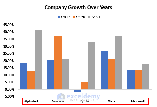
Consider the following dataset. It contains the annual growth of five U.S.-based companies. The letter Y before the years is used so that Excel considers them ...

Here's an overview of a doughnut chart with multiple rings, outlining sales data in different quarters. How to Create a Doughnut Chart with Multiple ...

This article deals with the excel area chart data label position. An area chart is used to plot data arranged in rows or columns on a worksheet. You can use it ...

What Is a Stacked Bar Chart? A stacked bar chart is a graph to represent and compare the segments of a whole. It can show the parts of a whole data ...

This article illustrates how to make a line graph in Excel with multiple variables. A line graph connects different data points to show the trend and make them ...
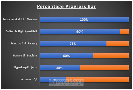
Dataset Overview Let's use the following dataset: Method 1 - Using a Bar Chart You can show the percentage progress bar by inserting a Bar Chart in ...

Step 1 - Downloading a Suitable Code 39 Barcode Font Close all of your office applications. Download the code 39 barcode font using the ...

Assume you have secured a loan of $1,000 at the annual rate of 14.49%. You can repay the loan in 12 equated monthly installments (EMI). Step 1 - ...

Step 1 - Set Leave Types and Months Make a list of the leave types that you allow for your employees. Assign a short code to each type for convenience. ...

Step 1- Set Budget Categories Enter the budget categories in B5:B10, here. Step 2 -Enter Budget Amounts Enter the expenses ...

This article illustrates how to automate consolidation in Excel. You can consolidate data from different worksheets or files in Excel. Data consolidation using ...

This article illustrates how to convert formula to value in multiple cells in excel. We usually use cell references in the formulas in Excel. Changing values ...

This article illustrates how to split inconsistent address in Excel. There are several ways to split consistent addresses in MS Excel. For example, the LEFT, ...
- « Previous Page
- 1
- …
- 3
- 4
- 5
- 6
- 7
- …
- 11
- Next Page »
See Our Reviews at


Thank you so much, Adam. We are really grateful to you for pointing it out. The article is updated.
Thanks & Regards
Md. Shamim Reza (ExcelDemy Team)
You can simply do that using any of the above methods that use the MIN function or the IF function.
1. MIN Function: The formula will be …
Total Grade = MIN(Exam_Grade + Extra_Credit*0.2,100)
2. IF Function: The formula will be …
Total Grade = IF(Exam_Grade + Extra_Credit*0.2>100,100,Exam_Grade + Extra_Credit*0.2)
Assume the Exam_Grade is in cell B2 and the Extra_Credit is in cell C2. Then apply any of the following formulas in cell D2 to get the Total_Grade with a maximum of 100.
=MIN(B2+C2*0.2,100)=IF(B2+C2*0.2>100,100,B2+C2*0.2)I have also emailed you an Excel document for this. Please check.
Thanks for reaching out to us.
Regards,
Md. Shamim Reza (ExcelDemy Team)
Thank you for your suggestion.
This should not happen with Filter. As soon as you clear the Filter, everything should be normal again. I suppose you SORTED the Products instead, excluding the Product Quantity. Then this becomes a complicated scenario.
I don’t know which Excel version you are using but you may try the following solutions. However, I can’t guarantee whether they will work for sure.
1. For Office365: Open the workbook. Go to File > Info > Version History. Check for any previous versions listed there. If not, then go to File > Info > Manage Workbook > Recovered Unsaved Workbooks. This will take you to the recovery folder for excel files. Look for a file with your workbook’s name.
2. For Excel 2019-2016: Open the Workbook. Go to File > History. Hopefully, you will find the previous versions listed there.
3. You can also check for any previous version using File Properties. Go to the file location. Right-click on the file name. Go to Properties > Previous Versions. Check for any previous versions listed there.
4. To manually check the recovery folder, go to File > Options > Save > Save Workbooks. Then copy the AutoRecover File Location and paste it on the File Explorer address bar.
You may visit this blog post from Microsoft for more >> https://support.microsoft.com/en-us/office/view-previous-versions-of-office-files-5c1e076f-a9c9-41b8-8ace-f77b9642e2c2
I hope you will be able to recover the file. Best of luck!
Thanks & Regards,
Md. Shamim Reza (ExcelDemy Team)
Hello Murali,
Unfortunately, I find your query a little confusing. It would’ve been much better if you had explained it with sample data and desired outputs.
As far as I understand, you need to compare column A in Book1 to column A in Book2. So, you want to create a formula in Book2 so that, if there is a match, it will return the corresponding value from column Z in Book1.
You can apply the following formula to do that. Then copy the formula down.
=IF(Sheet1!A1=[Book1.xlsx]Sheet1!A1,[Book1.xlsx]Sheet1!Z1,"")Is this what you wanted? I’ve also emailed you the Excel documents. Please check.
Thanks for being with us.
Regards,
Md. Shamim Reza (ExcelDemy Team)
Thanks for your input, Josh. You are absolutely right.
Regards,
Md. Shamim Reza (ExcelDemy Team)
Hi Joe,
Assume your example data table (with headers) starts from cell A1. The lower criteria range i.e 20 is in cell E2 and the upper criteria range i.e 30 in cell G2. Now enter the following formula in cell H2 to get the desired result.
=TEXTJOIN(",",TRUE,IF($B$2:$B$6>=$E$2,IF($B$2:$B$6<=$G$2,$C$2:$C$6,""),""))You can change the criteria ranges as required. For example, change the lower criteria from 20 to 25 and the upper criteria from 30 to 35. This will give you the #OFLANES values for the range 25-35. You can create dropdown lists in the criteria cells E2 and G2 to easily change the criteria value.
I’ve also emailed you an excel document with the solution. Please check.
Don’t hesitate to let us know if you face any further problems. Thanks for reaching out to us.
Regards,
Md. Shamim Reza (ExcelDemy Team)
Hello Robert,
I’ve checked the code again and it is working fine. Perhaps you haven’t used any wildcards and there was no exact match to the search value. Otherwise, you haven’t used the wildcards properly.
And can you please clarify what you mean by “variables are off”? Thanks.
Regards
Md. Shamim Reza (ExcelDemy Team)
Hi there,
I’ve applied your formula after correcting the typos (you’ve used semicolons instead of commas) and it is working fine.
=IFERROR(VLOOKUP(G$3&ROW($A$1:INDIRECT("A"&COUNTIF($C$4:$C$1276,G$3))),$B$4:$F$1403,3,FALSE),"")If you still face the problem, please explain it in detail so we can help you. Thanks for being with us.
Regards,
Md. Shamim Reza (ExcelDemy Team)
Hi Anya,
We regret to hear that. But you may have used the wrong shortcut. If you press ALT+W+H instead of ALT+H+W, then it will hide the window. Press ALT+W+U, then select the workbook in the popup window and click OK to unhide the window. Alternatively, you can click on Unhide from the Window group in the View tab.
I suggest you to make sure you are using the right shortcut before using any from next on. How can you do that? Well, if you press the Alt key, then you should see letters beside each tab on the Ribbon as the shortcut to go to that tab. Now press the letter visible beside the tab that you need to go. After that, you should see the shortcut letters visible beside each command on that tab. This way you will know if this is the right shortcut for the task.
Hope this solves your problem. If not then please let us know with details. We will try our best to help you fix that.
Regards
Md. Shamim Reza (ExcelDemy Team)
You can check the following code for that. Just copy the ElseIf statement for more columns.
Thanks for reaching out to us. Keep in touch.
Regards
Md. Shamim Reza (ExcelDemy Team)
Hi
You can check the following code for that. Just copy the ElseIf statement for more columns.
Thanks for reaching out to us. Keep in touch.
Regards
Md. Shamim Reza (ExcelDemy Team)
Hi Tony,
I couldn’t fully understand what you need from your comment. You said you want to retrieve information from Sheet1. But you are looking for information in the “RESULTS” sheet in all of those formulas that you’ve tried.
Can you share the workbook with us? Thanks.
Regards
Md. Shamim Reza (ExcelDemy Team)
Hi
I couldn’t understand the problem from your comment. Please explain what you need in details and share the workbook if possible. Then we will try our best to find you the solution.
Thanks for reaching out to us. Keep in touch.
Regards
Md. Shamim Reza (ExcelDemy Team)
Hi there!
I couldn’t fully understand what you need from your comment. However, I assumed you may want to create something like the following formula.
=IFERROR(IF(REPORT!A:C="OUTSTANDING","",VLOOKUP(B9,REPORT!A:C,3,FALSE)),"")Is this what you needed? If not, then tell us more about the problem so that we may help you. Thank you for being with us.
Regards
Md. Shamim Reza (ExcelDemy Team)
Hello Brian,
Thanks for reaching out to us. Well, you can ignore that step I think. Have you tried to run the code on your dataset?
Actually, I’d added the step because VBA was acting a little weird if there was a blank column at the beginning. Maybe because of the .EntireRow statement.
So, why don’t you run the code ignoring that step and see if it works? Thanks.
Regards
Md. Shamim Reza (ExcelDemy Team)
Hi Anil,
You are right. We normally use the “Set statement” to assign range objects. But it is done here indirectly without the Set statement.
This is a Change event. Here, “Target” indicates to all cells within the sheet. So the “For Each Cell In Target” statement works as the alternative to the Set statement.
Hope this clarifies your confusion. And thank you for reaching out to us.
Regards
Md. Shamim Reza (ExcelDemy Team)
Hi there!
I am assuming that you want the following result.
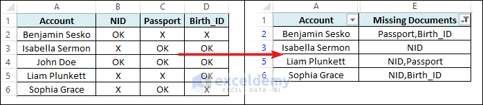
Then follow the steps below.
First, apply the following formula in cell E2 and copy it down.
=TEXTJOIN(",",TRUE,IF(B2:D2="X",$B$1:$D$1,""))Then, filter out the blank cells from column E.
Next, hide columns B to D.
Now you can print the summary data.
Please let us know if this is what you needed. If not then tell us more about it so that we may help. And thank you for being with us.
Regards
Md. Shamim Reza (Exceldemy Team)
Hi there!
You can use the GETPIVOTDATA function to do that. Find out more in the following articles.
https://www.exceldemy.com/compare-two-pivot-tables-in-excel/
https://support.microsoft.com/en-us/office/getpivotdata-function-8c083b99-a922-4ca0-af5e-3af55960761f
Thanks for being with us.
Regards
Md. Shamim Reza (Exceldemy Team)
Hi there!
I think the range is correct. Can you tell us why you think it is not? Thanks.
Regards
Md. Shamim Reza (Exceldemy Team)
Hi Paulino!
It is not clear from your comment whether you want all data consolidated in a single worksheet or to create a master workbook containing all worksheets from those files. I am assuming you want to do the latter as the datasets are completely different. Then follow the steps below.
First, open a new workbook and save it.
Then open any one of those files. Select the first sheet tab. Hold the SHIFT key and select the last sheet tab. This will select all sheets in that workbook.
Next, align the two workbooks side by side.
Then, drag the selected sheets to the master workbook. Now hold the CTRL key and drop the sheets beside the sheet tabs of the master workbook. After that, all the sheets from the file will be copied to the master workbook.
Now, open the other files one by one and repeat the procedures. Finally, you will get the master workbook containing all the sheets from those files.
Please let us know if you got that done by following the above steps. Thank you for being with us.
Regards
Md. Shamim Reza(Exceldemy Team)
Hello Steven!
We didn’t clearly understand your query. Can you tell us more about what you need? I assume from your comment that you may have found an alternate solution. Can you please share that with us? Thanks.
Regards
Md. Shamim Reza(Exceldemy Team)
Hi there!
We checked the formula. It is working fine. Make sure the absolute references are entered correctly. We suggest you download the file and practice there. You can tell us more about the problem if the formula isn’t still working for you.
And thank you for pointing out the error in the second step. We have corrected it.
Thank you again for being with us.
Regards
Md. Shamim Reza(Exceldemy Team)
Hello Grant!
Yes, you can do that. But if you gave a little more description of your dataset, it would’ve been easier for me to help you. Anyway, you can apply the following steps in Power Query for the dataset used in the 4th solution in the article.
Source = Excel.CurrentWorkbook(){[Name=”Table1″]}[Content]
Changed Type = Table.TransformColumnTypes(Source,{{“Roll”, Int64.Type}, {“Marks”, Int64.Type}})
Reordered Columns = Table.ReorderColumns(#”Changed Type”,{“Marks”, “Roll”})
Sorted Rows = Table.Sort(#”Reordered Columns”,{{“Marks”, Order.Ascending}})
Transposed Table = Table.Transpose(#”Sorted Rows”)
Merged Columns = Table.CombineColumns(Table.TransformColumnTypes(#”Transposed Table”, {{“Column1”, type text}, {“Column2”, type text}, {“Column3”, type text}, {“Column4”, type text}}, “en-US”),{“Column1”, “Column2”, “Column3”, “Column4”},Combiner.CombineTextByDelimiter(“,”, QuoteStyle.None),”Merged”)
Merged Columns1 = Table.CombineColumns(Table.TransformColumnTypes(#”Merged Columns”, {{“Column5”, type text}, {“Column6”, type text}, {“Column7”, type text}}, “en-US”),{“Column5”, “Column6”, “Column7”},Combiner.CombineTextByDelimiter(“,”, QuoteStyle.None),”Merged.1″)
Merged Columns2 = Table.CombineColumns(Table.TransformColumnTypes(#”Merged Columns1″, {{“Column8”, type text}, {“Column9”, type text}, {“Column10”, type text}}, “en-US”),{“Column8”, “Column9”, “Column10”},Combiner.CombineTextByDelimiter(“,”, QuoteStyle.None),”Merged.2″)
Merged Columns3 = Table.CombineColumns(Table.TransformColumnTypes(#”Merged Columns2″, {{“Column11”, type text}, {“Column12”, type text}}, “en-US”),{“Column11”, “Column12”},Combiner.CombineTextByDelimiter(“,”, QuoteStyle.None),”Merged.3″)
Transposed Table1 = Table.Transpose(#”Merged Columns3″)
Split Column by Delimiter = Table.SplitColumn(#”Transposed Table1″, “Column1”, Splitter.SplitTextByDelimiter(“,”, QuoteStyle.Csv), {“Column1.1”, “Column1.2”, “Column1.3”, “Column1.4″})
Changed Type1 = Table.TransformColumnTypes(#”Split Column by Delimiter”,{{“Column1.1”, Int64.Type}, {“Column1.2”, Int64.Type}, {“Column1.3”, Int64.Type}, {“Column1.4″, Int64.Type}})
Removed Columns = Table.RemoveColumns(#”Changed Type1”,{“Column1.2”, “Column1.3”, “Column1.4″})
Renamed Columns = Table.RenameColumns(#”Removed Columns”,{{“Column1.1”, “Marks”}, {“Column2”, “Roll”}})
Hello, Thomas!
You can apply the following formula in cell C14 to do that.
=TEXTJOIN(", ",,(VLOOKUP(LEFT(C13,(FIND(",",C13,1)-1))&"*",B5:C11,2)), (VLOOKUP(TRIM(RIGHT(C13, LEN(C13)-FIND(",",C13,1))&"*"), B5:C11,2)))**Notes:
1. If multiple results are associated with the lookup value, the formula will return the first result only.
2. You must enter at least 2 lookup values separated by comma. Otherwise, you may see #VALUE!
Regards
Shamim
Hello Kris! I am assuming that you are trying to do something as follows.
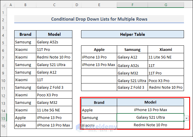
You can apply the following steps to be able to do that.
First, enter the following formula in cell E6.
=TRANSPOSE(SORT(UNIQUE(B5:B16)))Then, apply the following formula in cell E7.
=SORT(FILTER($C$5:$C$16,$B$5:$B$16=E$6))Next, drag the fill handle icon to the right.
After that, enter =$E$6# as the source for data validation in cell E14.
Then, drag the fill handle icon below.
Next, enter the following formula as the source for data validation in cell F14.
=INDIRECT(ADDRESS(7, COLUMN(D1) + MATCH(E14, $E$6#, 0), 4) & "#")Now copy the cell. Then select multiple cells below it. Next, paste it there as validation using paste special.
Hi Joe!
You are right. It is really difficult to understand the problem from the comment.
So, I’ve a requested you for the problematic document. Please check your email.
Regards
Shamim
Hi Chris, thanks for your query.
You are facing the issue probably because the defined range is dynamic. Besides, you shouldn’t use the same defined range as the ListFillRange for multiple combo boxes. Rather you need to create a unique defined range for each of the combo boxes. You may try the following solution.
First, change the source of the defined range named as Dropdown_List to =States!$E$5:$E$17.
Then, enter the following formula in cell F5 in the States worksheet.
=FILTER(B5:B17,ISNUMBER(SEARCH(Dropdown!G4,B5:B17)),”Not Found”)
Next, create a new defined range and name it as Dropdown_List2 and enter =States!$F$5:$F$17 in the source field.
Now, insert another ComboBox in the Dropdown sheet and link it to cell G4. Enter Dropdown_List2 as the ListFillRange for this ComboBox.
After that, open the VBA window and replace the earlier code with the following one.
Private Sub ComboBox1_Change()
ComboBox1.ListFillRange = “Dropdown_List”
Me.ComboBox1.DropDown
End Sub
Private Sub ComboBox2_Change()
ComboBox2.ListFillRange = “Dropdown_List2”
Me.ComboBox2.DropDown
End Sub
Finally, run the code and hopefully you won’t face the issue again.
Walaikum Assalam, KJ. Thanks for your query.
You can try the following code. The pictures will be copied to the next column.
Then, you can resize them and right-click to save them as pictures.
Alternatively, you can copy the worksheet or the workbook and save it as Web Page (*.htm, *.html).
Then, all of the pictures will be saved to a new folder (named after the file) in the same location as the saved file.
Glad to hear that. You are welcome!
Glad to know that. You are welcome!
Thank you very much for your suggestion. Good to know that.
Hopefully, this will help someone.
And Good Luck to you too!
Thank you very much for your feedback, Hermann.
Great suggestion! Will keep in mind.