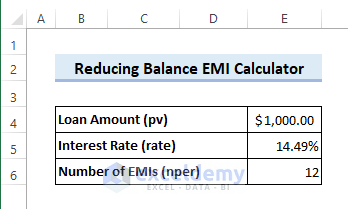
Assume you have secured a loan of $1,000 at the annual rate of 14.49%. You can repay the loan in 12 equated monthly installments (EMI).
Step 1 – Calculate EMI Amount with PMT Function
- Enter the following formula in cell E8 to estimate the EMI amount. Here the PMT function returns negative numbers. Therefore a negative sign has been used at the beginning of the formula.
=-PMT(E5/12,E6,E4,0,0)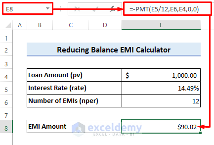
Step 2 – Estimate Total Amount Payable
- Enter the following formula in cell E9 to calculate the total payable amount:
=E8*E6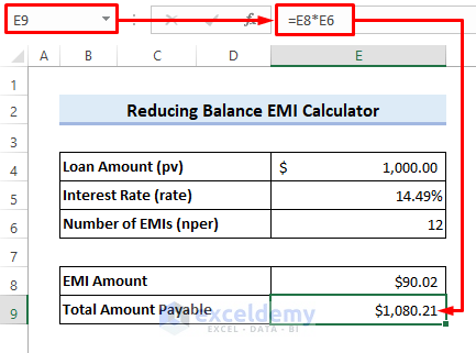
Step 3 – Calculate Total Interest
- Enter the following formula in cell E10 to get the total interest:
=E9-E4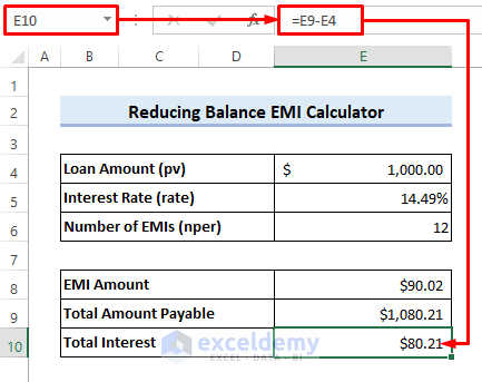
Read More: Home Loan EMI Calculator with Reducing Balance in Excel
Step 4 – Create a Reducing Balance EMI Table
- Input 1 to 12 in cells B13 to B24, respectively.
- Insert the following formula in cell C13:
=E4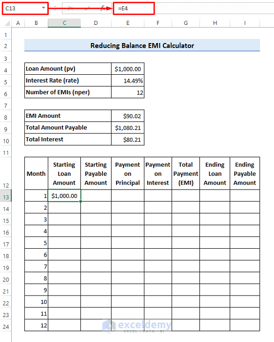
- Enter the following formula in cell D13:
=E9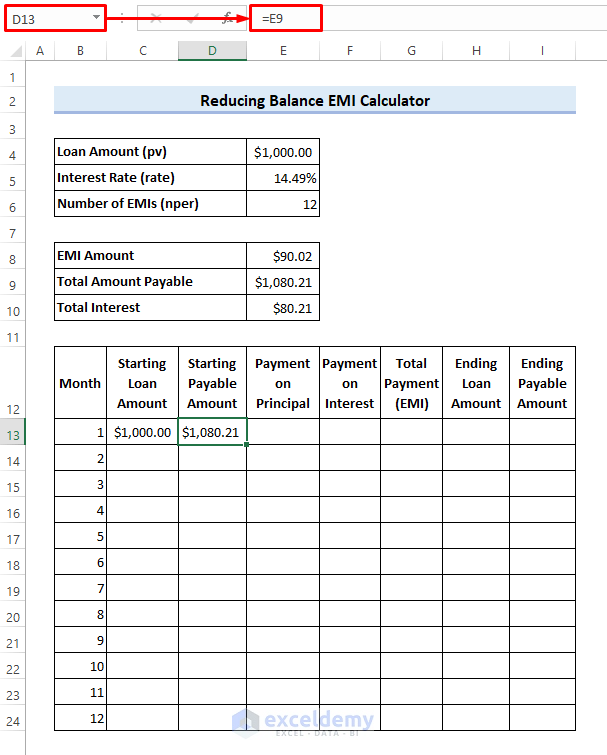
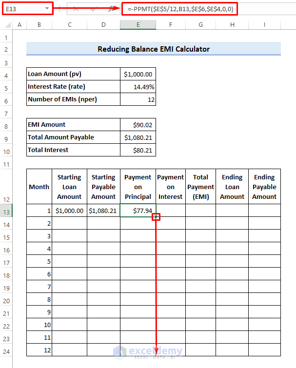
- Apply the following formula in cell E13 to calculate the monthly payment need to be made on the principal loan amount.
=-PPMT($E$5/12,B13,$E$6,$E$4,0,0)- Drag the Fill Handle icon down to cell E24. Here, the PPMT function also returns negative values as it considers the payment as cash outflow.
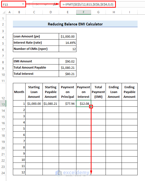
- Enter the following formula in cell F13 to calculate the monthly payment need to be made on the interest:
=-IPMT($E$5/12,B13,$E$6,$E$4,0,0)
- Drag the Fill Handle icon down to cell F24. Here, the IPMT function also considers the payments as cash outflow. So a negative sign is used at the beginning to avoid a negative result.
- Enter the following formula in cell G13 to calculate the total monthly payment. You can see that the result is equal to the EMI amount.
=SUM(E13:F13)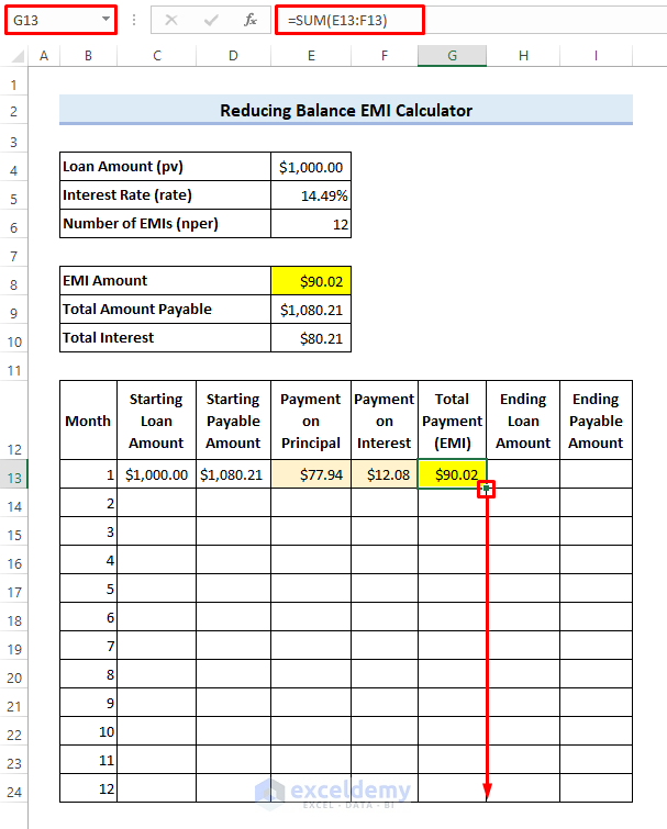
- Enter the following formula in cell H13 to calculate the remaining loan balance at the end of the month, then drag the Fill Handle icon down to cell H24.
=C13-E13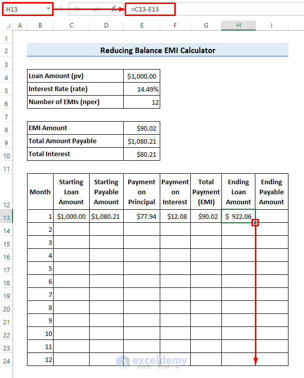
- Enter the following formula in cell I13 to calculate the total amount payable at the end of the month and drag the Fill Handle icon down to cell I24.
=D13-G13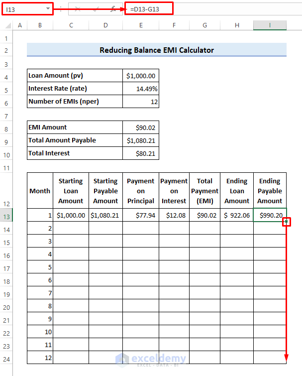
- Enter the following formula in cell C14 and drag the Fill Handle icon down to cell C24:
=H13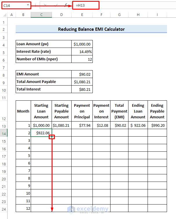
- Use the following formula in cell D14 and drag the Fill Handle icon down to cell D24.
=I13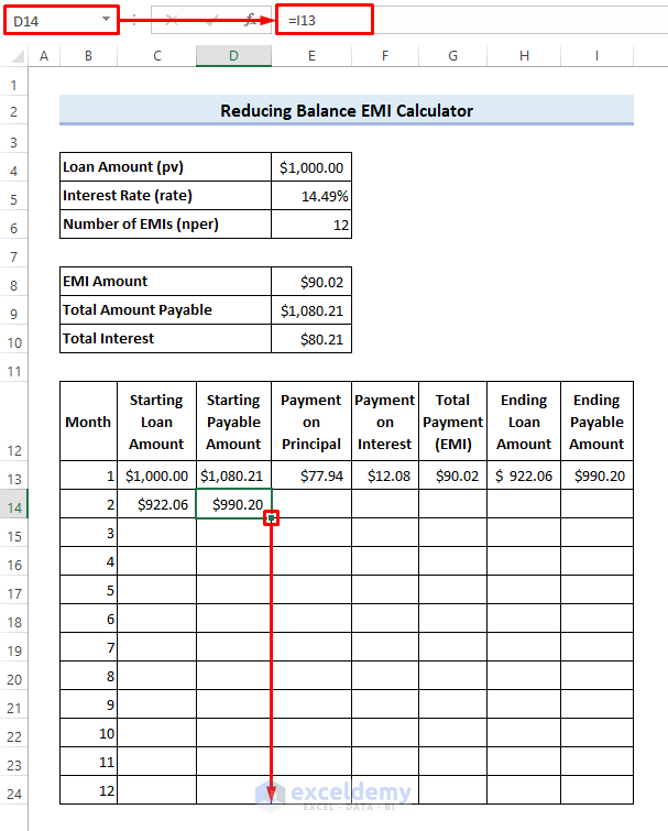
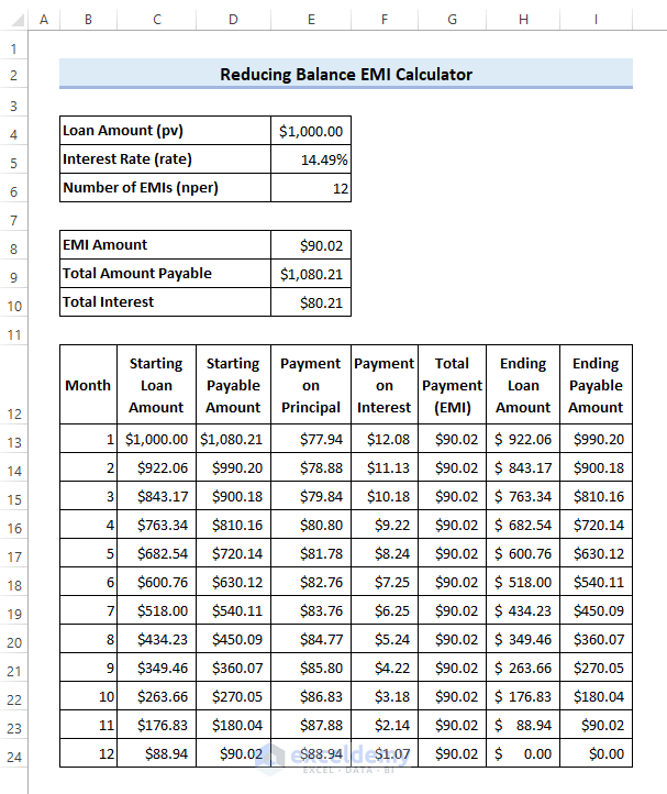
Step 5 – Finalize the EMI Calculator Sheet
- You will see the following result.
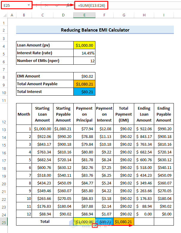
- Enter the following formula in cell E25 to verify the results.
=SUM(E13:E24)- Drag the Fill Handle icon to cell G25.
- You will see that the total payment made on the loan, the total payment made on interest, and the total amount payable match the results calculated earlier.
Note:
Don’t forget to use a negative sign before the formulas containing the financial function to avoid any negative results.
Read More: How to Create Reverse EMI Calculator in Excel
Download the Sample Workbook
Related Articles
- Personal Loan EMI Calculator Excel Format
- SBI Home Loan EMI Calculator in Excel Sheet with Prepayment Option
- Create Home Loan EMI Calculator in Excel Sheet with Prepayment Option
- EMI Calculator with Prepayment Option in Excel Sheet
<< Go Back to EMI Calculator | Finance Template | Excel Templates
Get FREE Advanced Excel Exercises with Solutions!

Thank you so much. I’d like to learn more from you. I believe all the solutions I’m looking for will be found here. Much love.
Hello Cosmas Gabu,
You’re most welcome! I’m so glad you found the content helpful. Keep exploring website, there are plenty of tutorials and guides to help you with your learning journey. If you have any questions or topics you’d like to learn more about, feel free to ask. Much love and happy learning!
You will get all article category and list here: Learn Excel
Regards
ExcelDemy