An Equated Monthly Installment (EMI) represents the amount to be paid every month to the bank or another financial institution. Over time, EMIs cover both the principal loan amount and the interest. EMIs are commonly used for various types of purchases across different sectors. To calculate EMIs accurately, EMI calculators are essential tools. In this tutorial, we’ll create a home loan EMI calculator with a reducing balance in Microsoft Excel.
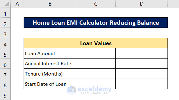
Step 1 – Set Up the Loan Value Dataset
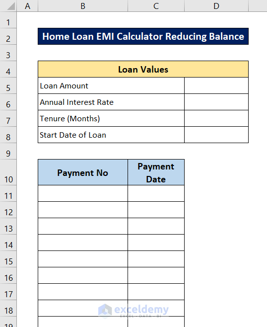
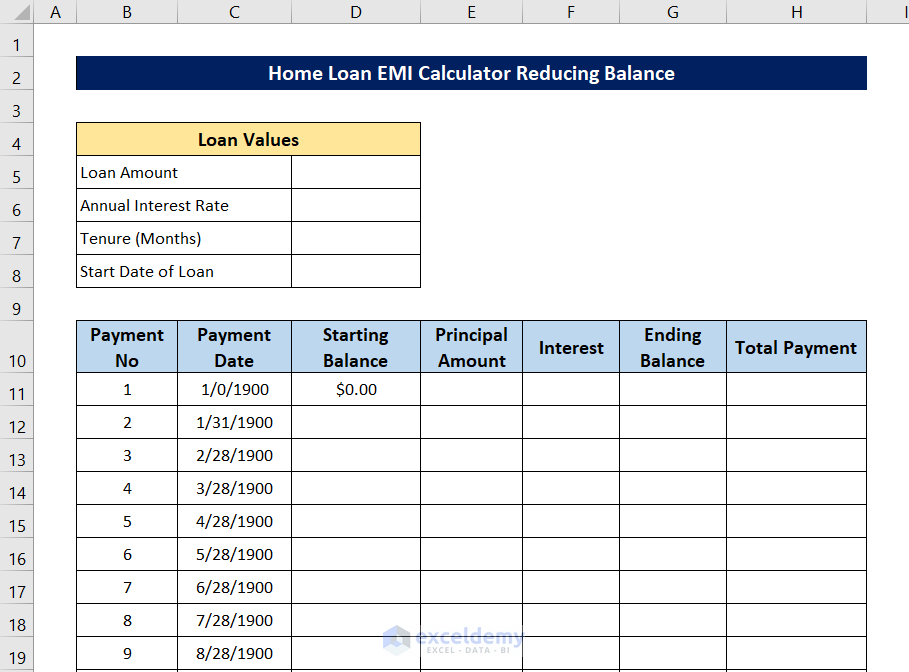
- Create the input section for the home loan EMI calculator. This section should include fields for the loan amount, down payment, insurance, interest rate, loan duration (in months), and start/end dates.
- Format the cells as follows:
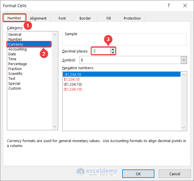
- Cell D5 (Loan Amount): Insert the Currency format with two decimal places.
- Press Ctrl+1 to open up the Format Cells
- Select the Currency format from the Number tab and select the preferred decimal places.
- Click OK.
- Cell D5 (Loan Amount): Insert the Currency format with two decimal places.
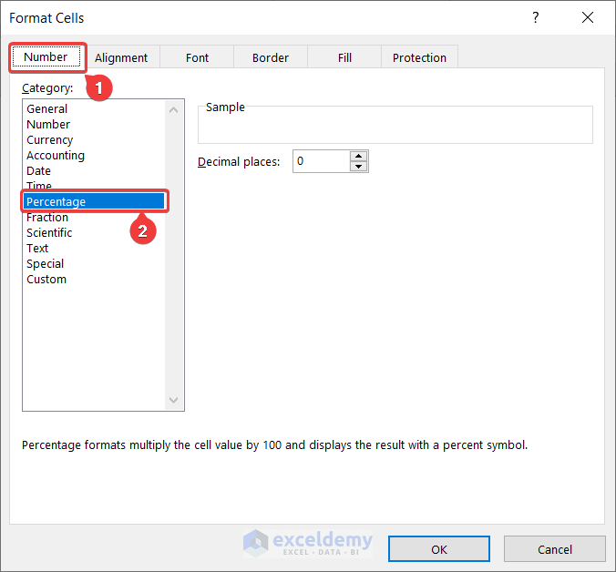
- Cell D6 (Interest Rate): Use the Percentage format.
- Press Ctrl+1 on your keyboard.
- Select the Percentage format from the Number tab.
- Click OK.
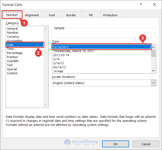
- Cell D8 (Start Date): Insert the desired date format.
- Press Ctrl+1 on your keyboard.
- Select the Date format from the Number tab in the Format Cells box and select the date type you prefer.
- Click OK.
Now our input section is ready for further calculations.
Step 2 – Construct Columns for Payment Number and Date
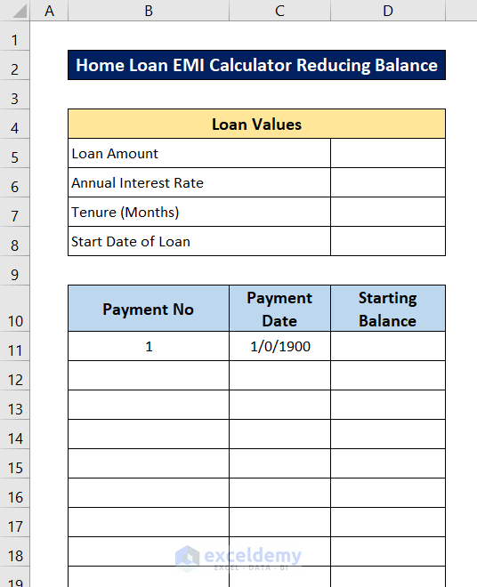
- Add columns to track payment numbers and due dates below the input section.
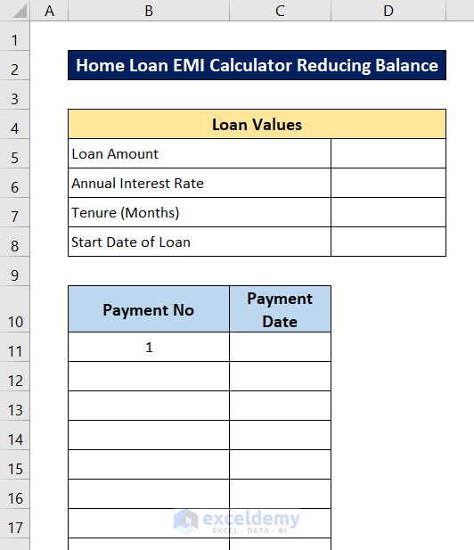
- In cell B11, enter “1” to start the payment tracking.
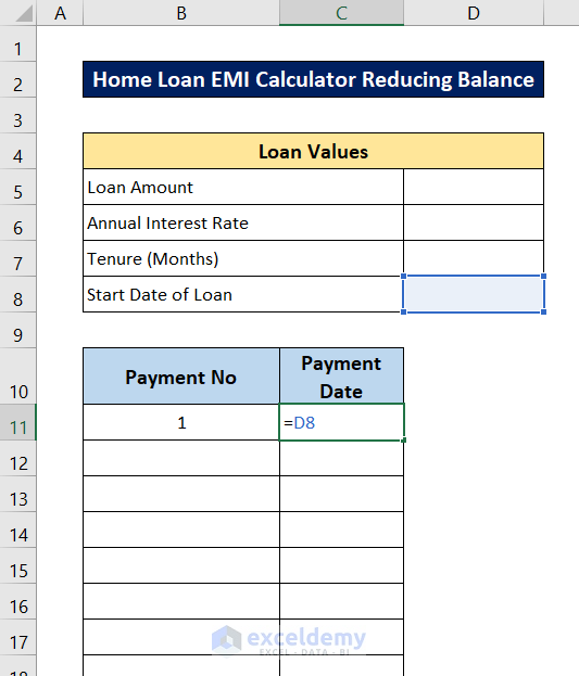
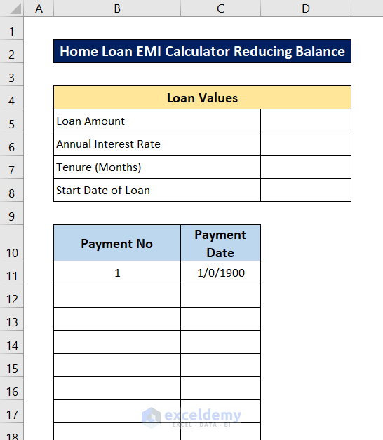
- In cell C11, insert the following formula to set the due date for the first payment.
=D8
Below indicates what the payment tracking section should look like:
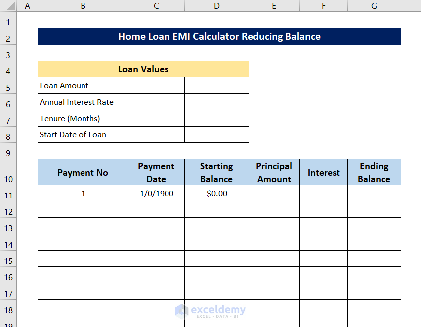
Step 3 – Calculate Starting Balance for Each Payment
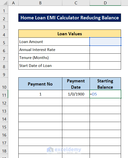
- Create a new column labeled Starting Balance in the dataset.
- In cell D11, insert the following formula to calculate the starting balance for the first payment:
=D5
As a result, the starting balance of the first payment will be populated.
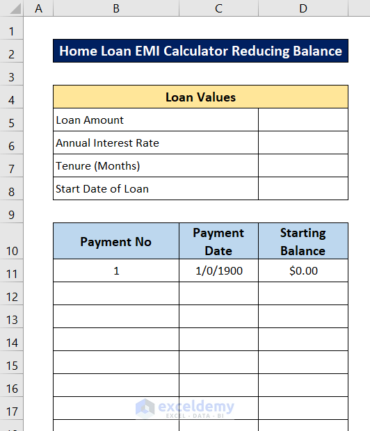
Note that the amount will be 0 initially due to blank input cells in the upper chart.
Read More: Create Home Loan EMI Calculator in Excel Sheet with Prepayment Option
Step 4 – Determine Principal Amount for Each Payment
- Create a column for the principal amount calculation.
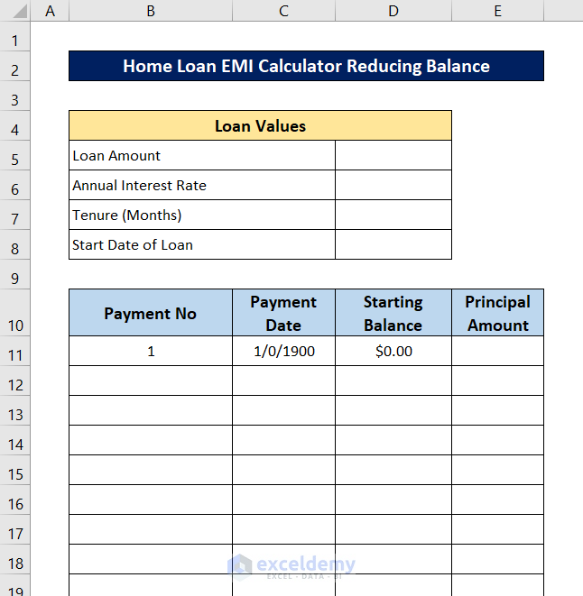
- In cell E11, insert the following formula:
=IFERROR(IF(B11="","",-PPMT($D$6/12,B11,$D$7,$D$5)),"")
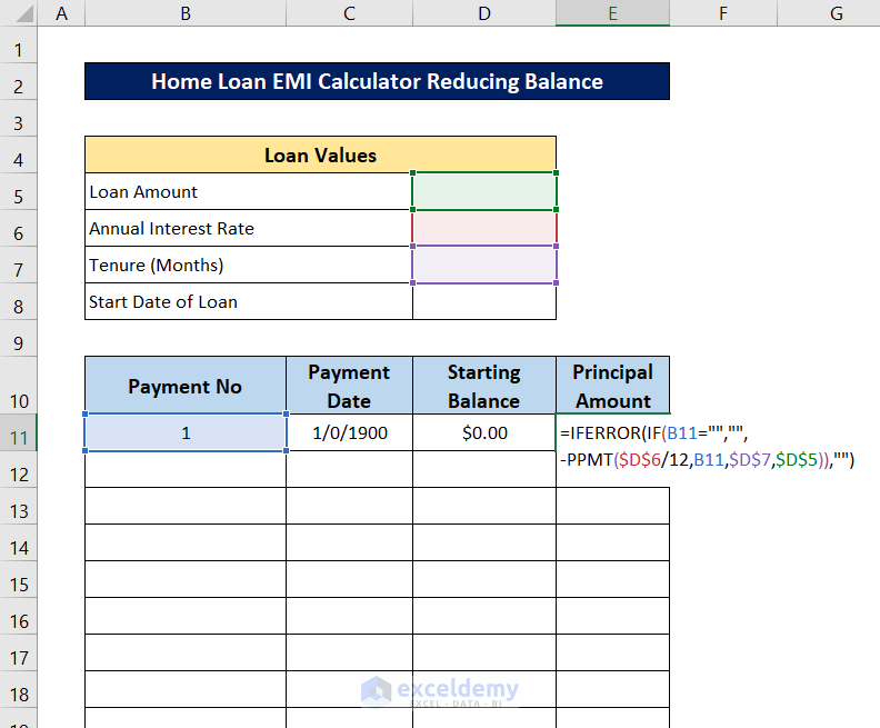
- Press Enter. This formula calculates the principal amount for the first payment.

The output here is blank because the cell references of the input values are blank.
Breakdown of the formula
IFERROR(IF(B11=””,””,-PPMT($D$6/12,B11,$D$7,$D$5)),””)
-PPMT($D$6/12,B11,$D$7,$D$5):
- This part calculates the principal amount of the payment.
- It uses the following inputs:
- Annual interest rate (cell D6), divided by 12 to get the monthly rate.
- Current period number (cell B11).
- Total number of periods (cell D7).
- Principal loan amount (cell D5).
- The result is negative because it represents an outflow (payment).
IF(B11=””,””,-PPMT($D$6/12,B11,$D$7,$D$5):
- This portion checks if cell B11 is blank.
- If B11 is blank, it returns a blank value; otherwise, it returns the principal amount calculated in the previous step.
Finally, IFERROR(IF(B11=””,””,-PPMT($D$6/12,B11,$D$7,$D$5)),””):
- This formula prevents errors from displaying.
- If any part of the formula encounters an error, it returns a blank value.
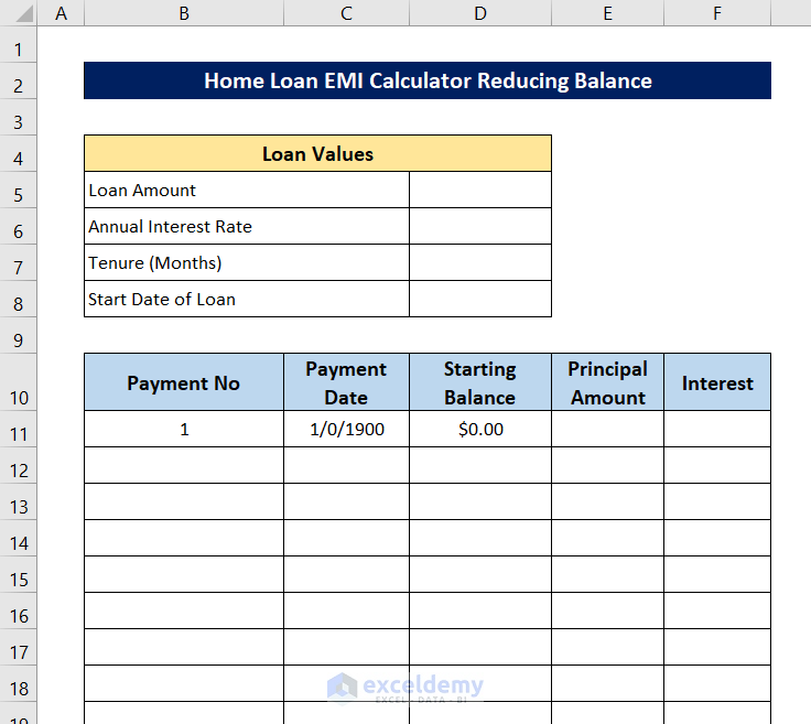
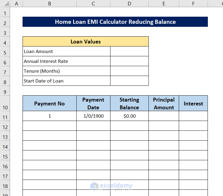
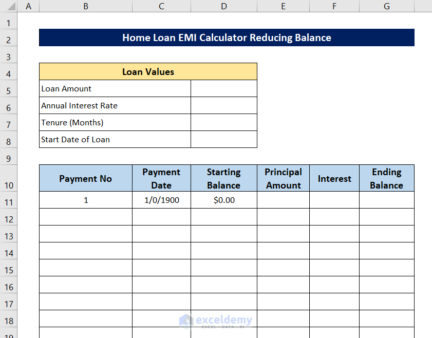
Step 5 – Compute Interest for Each Payment
Let’s calculate the interest for each payment using the IPMT function. We’ll also handle errors to keep our reducing balance chart clean.
- Create a new column for interest calculations.
- In cell C11, insert the following formula:
=IFERROR(IF(B11="","",-IPMT($D$6/12,B11,$D$7,$D$5)),"")
-
- The IPMT function considers the same inputs as before but calculates interest payments.
- We add a minus sign to make the result positive (for presentation purposes).
- The IFERROR part handles any errors that may occur during execution.
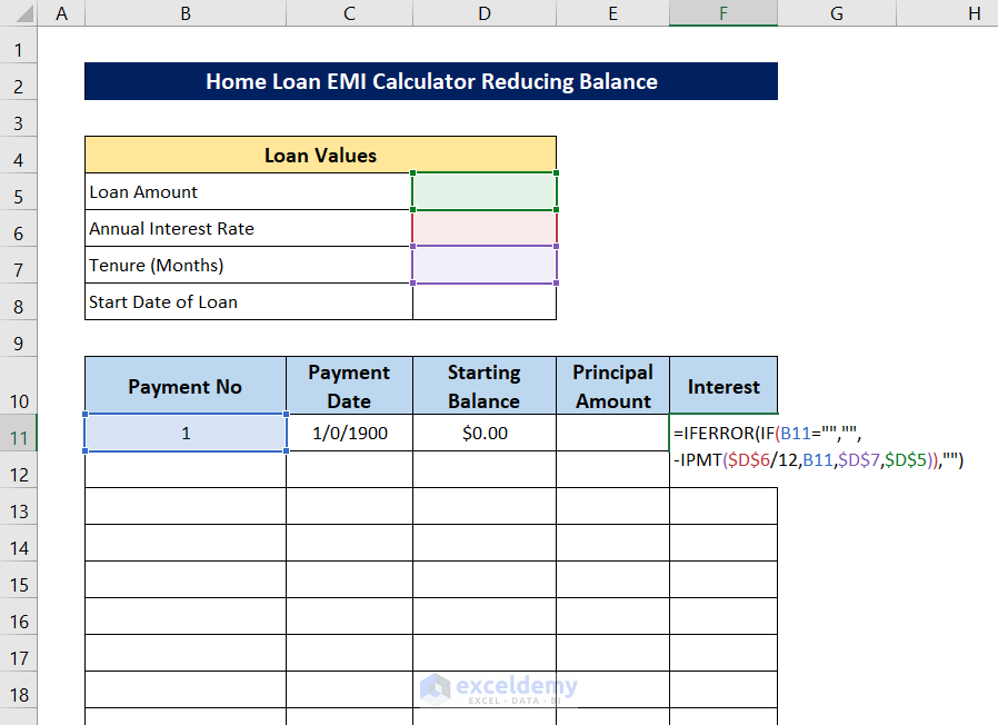
- Press Enter. The cell will appear blank for now since there are no values for the IPMT function.
Breakdown of the Formula
IFERROR(IF(B11=””,””,-IPMT($D$6/12,B11,$D$7,$D$5)),””)
IPMT($D$6/12,B11,$D$7,$D$5):
- This part calculates the interest payment for each period.
- It uses the following inputs:
- Annual interest rate (cell D6), divided by 12 to get the monthly rate.
- Current period number (cell B11).
- Total number of periods (cell D7).
- Principal loan amount (cell D5).
- The result is negative because it represents an outflow (payment).
IF(B11=””,””,-IPMT($D$6/12,B11,$D$7,$D$5)):
- This portion checks if cell B11 is blank.
- If B11 is blank, it returns a blank value; otherwise, it returns the interest amount calculated in the previous step.
IFERROR(IF(B11=””,””,-IPMT($D$6/12,B11,$D$7,$D$5)),””):
- This formula prevents errors from displaying.
- If any part of the formula encounters an error, it returns a blank value.
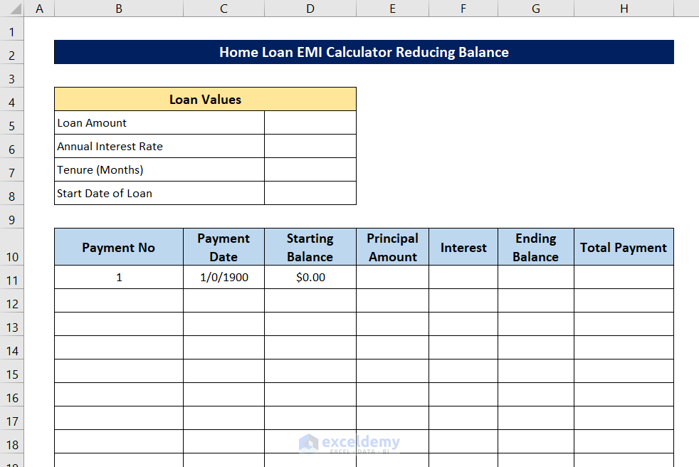
Step 6 – Calculate Ending Balance After Each Payment
- Create a new column next to our reducing balance chart.
- In cell G11, insert the formula:
=IFERROR(IF(B11="","",D11-E11),"")
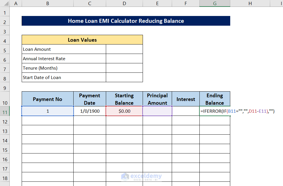
- Press Enter.
- This formula calculates the ending balance after paying the EMI for the respective month.
- The result will be blank initially due to zero or blank cell references.
Breakdown of the Formula
=IFERROR(IF(B11=””,””,D11-E11),””)
IF(B11=””,””,D11-E11):
- This function checks whether cell B11 is blank.
- If B11 is blank, it returns a blank value; otherwise, it calculates the difference between the values in cells D11 and E11.
IFERROR(IF(B11=””,””,D11-E11),””):
- This formula handles errors.
- If any part of the formula encounters an error, it returns a blank string.
Read More: SBI Home Loan EMI Calculator in Excel Sheet with Prepayment Option
Step 7 – Compute Total Amounts Paid
- Create a new column where we can calculate and record the total amounts paid for each EMI.
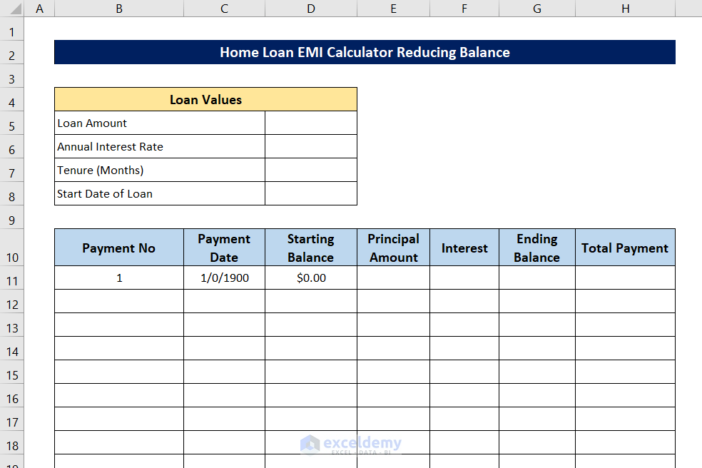
- Select cell H11 and enter the following formula:
=IFERROR(IF(B11="","",E11+F11),"")
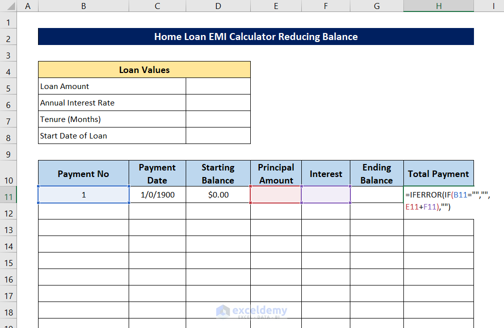
- Press Enter to calculate the total payment of the first transaction. For now, the cell is empty because the cell references that the formula used is empty.
Breakdown of the Formula
IFERROR(IF(B11=””,””,E11+F11),””)
IF(B11=””,””,E11+F11):
- This formula checks if the value in cell B11 is blank or not.
- If it is blank, then the function returns blank. This helps the numbers to stop repeating when the chart ends.
- If the cell value of B11 is not empty, it returns the sum of cells E11 and F11 as the output.
IFERROR(IF(B11=””,””,E11+F11),””):
- Checks for an error in the inner function.
- If there were any errors, it returns an empty string instead of showing the error.
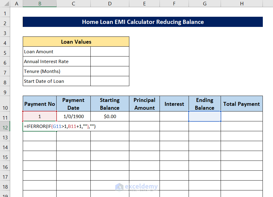
Step 8 – Replicate Formulas for Later Rows
- Up until now, we’ve only created formulas in the first row. We need to replicate these formulas for subsequent rows.
- Select cell B12 and enter the following formula:
=IFERROR(IF(G11>1,B11+1,""),"")
Breakdown of the Formula
IFERROR(IF(G11>1,B11+1,””),””)
IF(G11>1,B11+1,””):
- This formula checks if the value in cell G11 is greater than 1.
- If true, it returns a value one greater than that of cell B11 (incrementing the payment number).
- Otherwise, it returns a blank value.
IFERROR(IF(G11>1,B11+1,””),””)
- Checks for an error in the inner function.
- If there were any errors, it returns an empty string instead of showing the error.
- Press Enter.
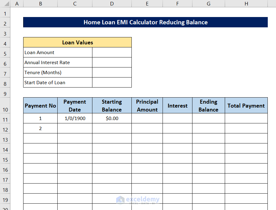
- Drag the fill handle down to populate this formula for a large number of rows.
- Select cell C12 and insert the following formula.
=IF(B12="","",EDATE(C11,1))
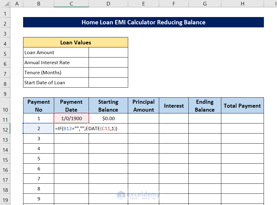
Breakdown of the Formula
IF(B12=””,””,EDATE(C11,1))
EDATE(C11,1):
- Takes the value of cell C11 as the initial month argument and returns the value of the exact date of the next month.
IF(B12=””,””,EDATE(C11,1)):
- Checks if there are any missing value in the previous cell (cell B12). If the value is empty, it returns an empty string. Otherwise, it executes the previous function.
- Press Enter.
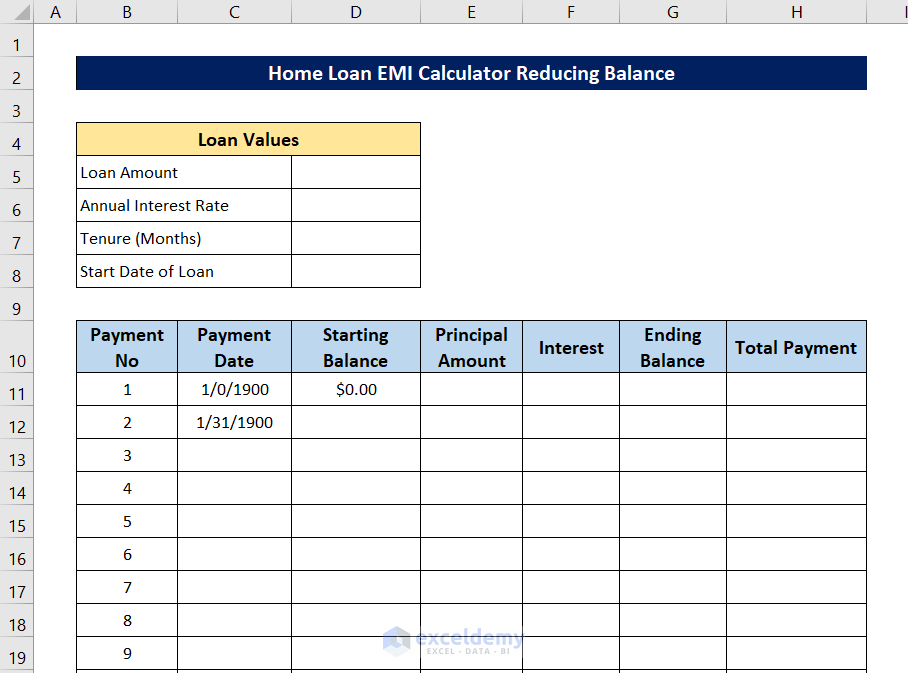
- Select the cell again and double-click the Fill Handle icon to automatically fill up the values for the rest of the cells.
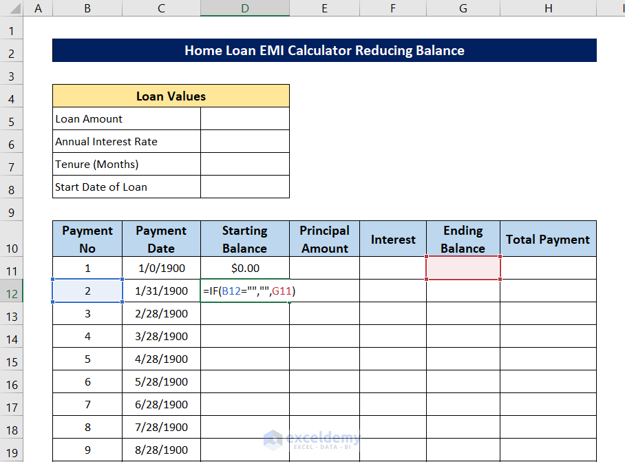
- For the “Starting Balance,” select cell D12:
=IF(B12="","",G11)
-
- This formula ensures that the starting balance continues from the previous row.
- The cell will remain blank until there’s a value in cell G11.
- Press Enter.
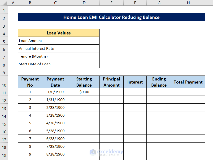
- To replicate formulas for the “Principal Amount”, “Interest”, “Ending Balance”, and “Total Payment” columns, select the range E11:H11 and double-click the fill handle icon.
The reducing balance chart for a home loan EMI calculator in Excel is now complete.
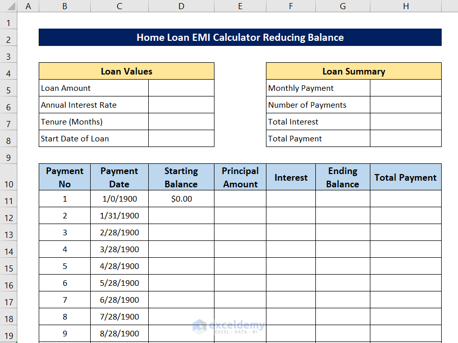
Step 9 – Generate Loan Summary
- Create a chart with the specified parameters.
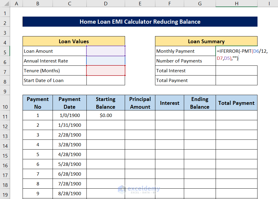
- In cell H5, enter the following formula:
=IFERROR(-PMT(D6/12,D7,D5),"")
Breakdown of the Formula
IFERROR(-PMT(D6/12,D7,D5),””)
PMT(D6/12,D7,D5):
- Calculates the loan payment for each transaction, using 1/12th of the interest rate (cell D6), the total number of payment periods (cell D7), and the principal amount (cell D5).
- The negative sign before the function ensures a positive value for the summary.
IFERROR(-PMT(D6/12,D7,D5),””):
- Prevents error warnings by returning an empty string if any errors occur.
- Press Enter to calculate the monthly payment for each EMI.
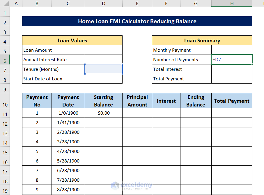
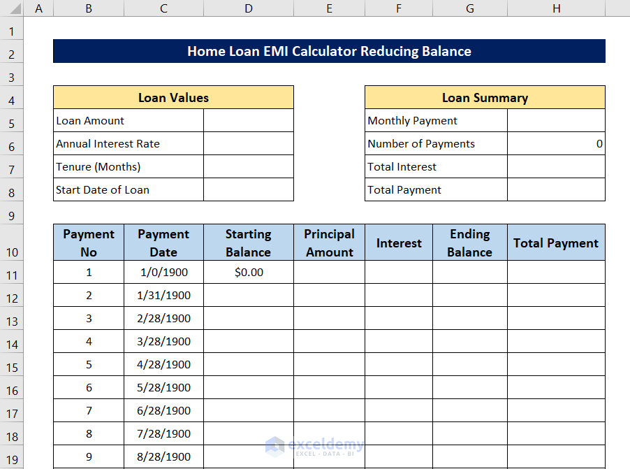
- In cell H6, enter the following formula and press Enter:
=D7
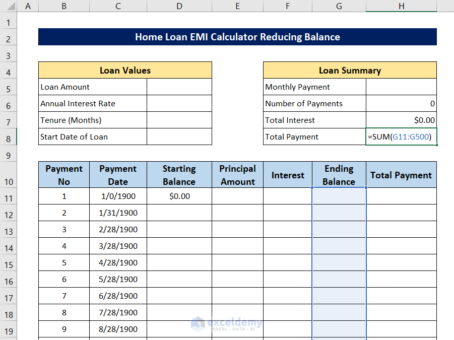
- In cell H7 enter the following formula:
=SUM(H11:H500)
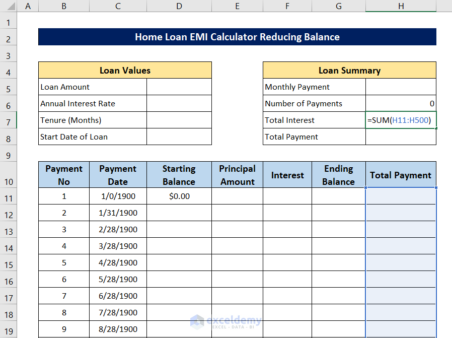
- Press Enter to get the total payment.
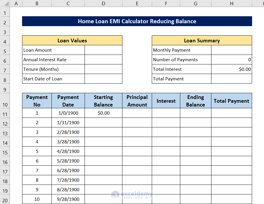
- In cell H8 and enter the following formula.
=SUM(G11:G500)
- Press Enter to calculate the total principal paid.
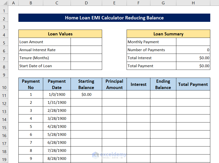
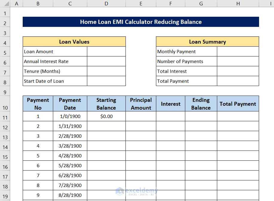
The home loan EMI calculator with the reducing balance chart in Excel is now complete.
Step 10 – Verify Home Loan EMI Calculator with Data
- Enter the following values in the appropriate sections under Loan Values:
- Loan amount: $400,000
- Annual interest rate: 5%
- Loan tenure: 5 years (60 months)
- Loan start date: 20th June 2022
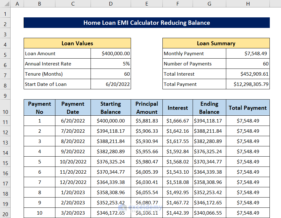
- Check that the payment and payment dates match the reducing balance chart.
- Confirm that both the monthly payment in the Loan Summary section and the reducing balance chart align.
- If everything matches, your calculator is working correctly.
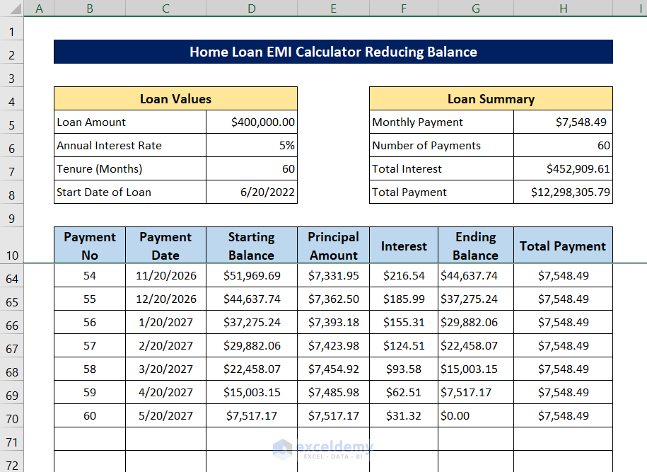
Go down the reducing balance chart and verify that the payments ended at the 60th transaction, if yes then the calculator gives the exact number of transactions.
Download Practice Workbook
You can download the practice workbook from here:
Related Articles
- Personal Loan EMI Calculator Excel Format
- Reducing Balance EMI Calculator in Excel Sheet
- EMI Calculator with Prepayment Option in Excel Sheet
- How to Create Reverse EMI Calculator in Excel
<< Go Back to EMI Calculator | Finance Template | Excel Templates
Get FREE Advanced Excel Exercises with Solutions!
