This is an overview:
Method 1 – Using the Goal Seek Feature to Create a Reverse EMI Calculator in Excel
Step 1: Establishing the Relationship
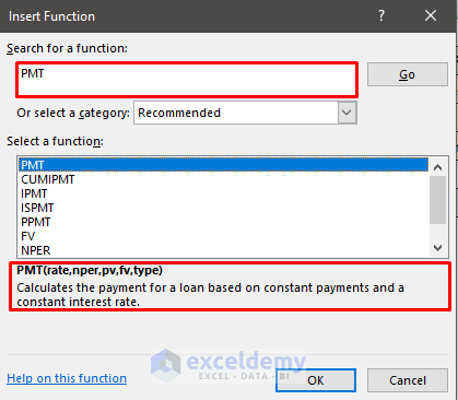
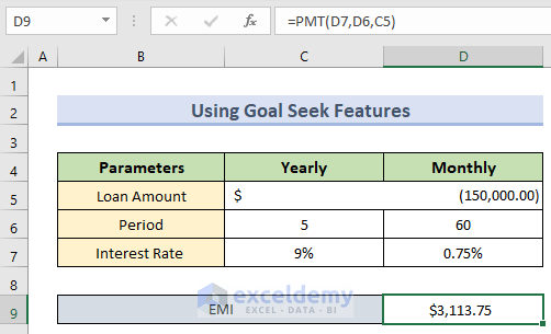
To establish the relationship between the EMI and the Total Loan based on the Interest Rate and Time, use the PMT function. Its syntax is:
=PMT(rate,nper,pv,fv,type)
- Enter the total time (nper) and interest rate (rate).
- Use the following formula:
=PMT(D7,D6,C5)
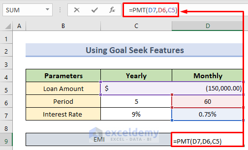
- Press Enter to see the result.
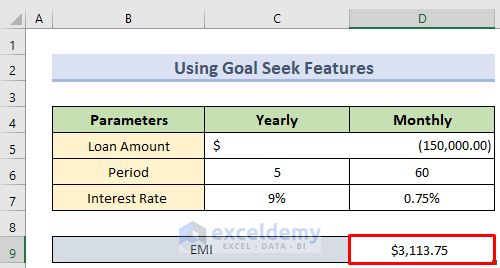
The EMI is calculated.
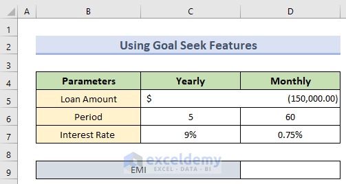
Step 2: Setting up the Parameters
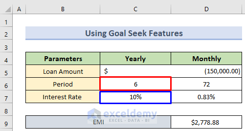
Change the npr and the rate. Here, a time period of 6 years at a rate of 10%.
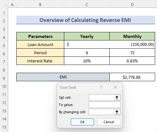
Step 3: Using the Goal Seek Feature to Calculated the Reverse EMI
- Go to the Data tab and select What If Analysis in Forecast.
- Select Goal Seek.
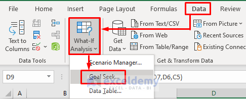
- In the Set cell, enter the EMI amount.
- In By changing cell, select the cell containing the total Loan Amount.
- Press Enter.
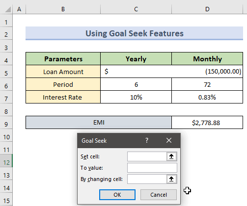
The EMI was set to 3000$ to see the total amount or present value.
2. Using the PV Function to Create a Reverse EMI Calculator in Excel
Steps:
- To find the Loan Amount in the dataset below:
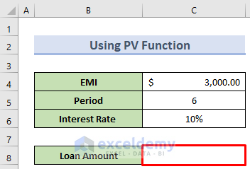
- Select a cell to see the output and enter the following formula in the formula bar:
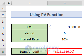
=PV(C6/12,C5*12,C4)
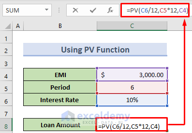
- Press Enter to see the result.
Read More: Reducing Balance EMI Calculator in Excel Sheet
Things to Remember
- The Goal Seek feature requires an existing relationship.
Download Practice Workbook
Download the following workbook.
Related Articles
- Personal Loan EMI Calculator Excel Format
- Home Loan EMI Calculator with Reducing Balance in Excel
- Create Home Loan EMI Calculator in Excel Sheet with Prepayment Option
- SBI Home Loan EMI Calculator in Excel Sheet with Prepayment Option
- EMI Calculator with Prepayment Option in Excel Sheet
<< Go Back to EMI Calculator | Finance Template | Excel Templates
Get FREE Advanced Excel Exercises with Solutions!
