What Is Home Loan EMI?
EMI stands for Equated Monthly Installment. It includes repayment of the principal amount and payment of the interest on the outstanding amount of your home loan. The formula for calculating the home loan EMI is.
Here,
P = Principal Loan Amount
N = Loan Tenure in months
R = Rate of Interest
As you repay the loan, you’re repaying a part of the principal (the money you loaned) plus the accumulated interest.
SBI Home Loan EMI Calculator in Excel Sheet with Prepayment Option: Create with Easy Steps
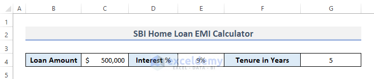
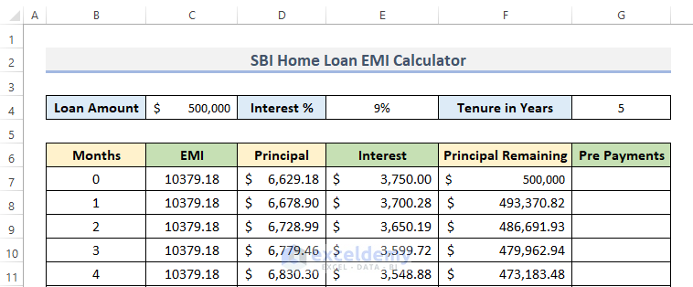
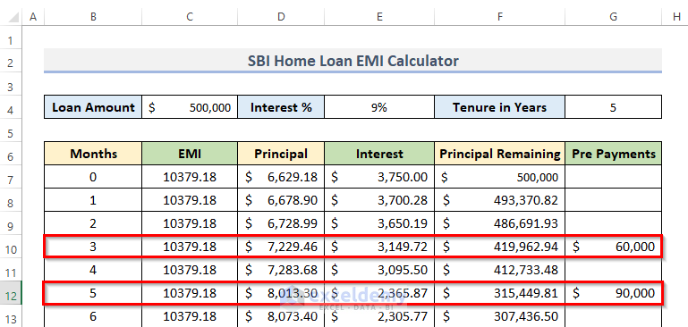
Step 1 – Insert Loan Amount, Interest Rate, and Tenure in Years
Put the basic information for further calculation.
- Insert the information on the Loan Amount. For example, we put our loan amount at $500,000.
- Set the Interest rate. In our case, the percentage is 9.
- Put the Tenure in Years – payback term. This is the amount of time that we have to return our total home loan, including interest. We put 5 years.
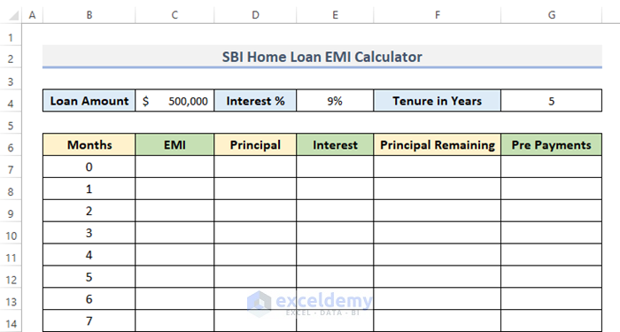
Step 2 – Set Months and Principal Remaining
As the tenure is 5 years, so the repayment will be done over 5*12 = 60 months.
- Create columns for Months, EMI, Principal, Interest, Principal Remaining, and Prepayments.
- Input the numbers of months in the Months column.
- Choose cell B7 and type 0.
- Drag the Fill Handle down to cell B67.
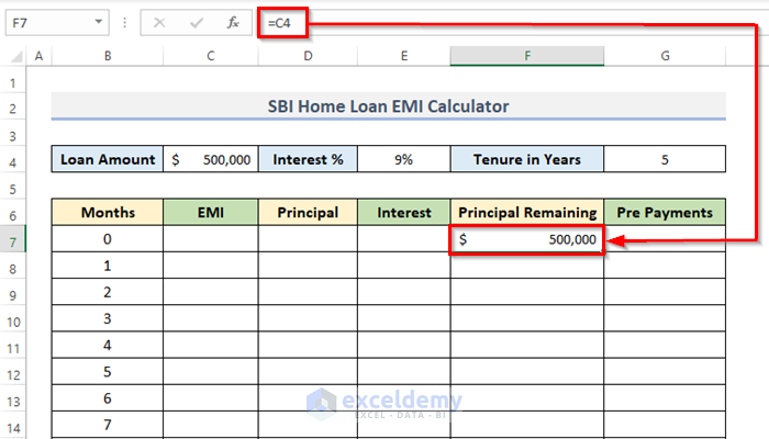
- Put the first Principal Remaining amount which is the Loan Amount (put in cell C4).
Read More: EMI Calculator with Prepayment Option in Excel Sheet
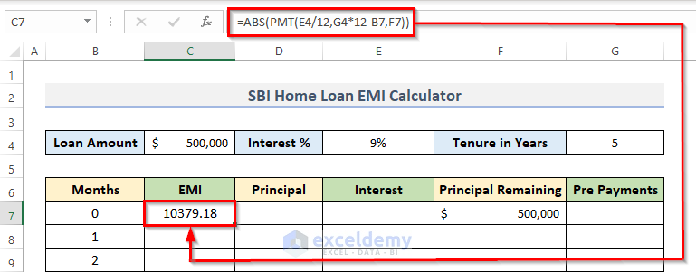
Step 3 – Calculate Equated Monthly Installment (EMI)
- Select cell C7 and put this formula to calculate EMI:
=ABS(PMT(E4/12,G4*12-B7,F7))- Press Enter to see the result:
How Does the Formula Work?
The Monthly Interest Rate is the first input (E4/12). Then, The number of months left is indicated by the second input (G4*12-B7). After that, The Remaining Principal Amount is represented by the third parameter (F7).
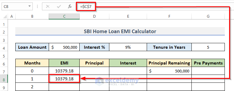
The EMI for other months will be the same. This will be fixed for the rest of the month. So, we put the previous cell in for the first month but with the absolute reference.
Step 4 – Compute Interest Amount
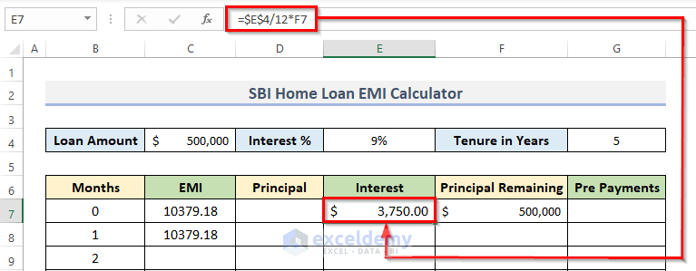
- Select cell E7 and insert this formula into that selected cell:
=$E$4/12*F7- Press Enter to see the result.
How Does the Formula Work?
To obtain the monthly interest rate in this calculation, we divided the annual interest rate by 12. Afterward, to calculate the interest amount, multiply it by the remaining principal amount.
Read More: Home Loan EMI Calculator with Reducing Balance in Excel
Step 5 – Calculate Monthly Principal and Principal Remaining
- Select a cell and put the formula into that cell. We used D7.
=C7-E7- Hit Enter.
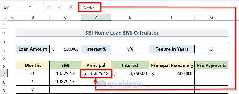
Here, we substract the Interest Amount from Equated Monthly Installment (EMI) to get the Principal Amount.
- Select the first month of principal remaining.
- Insert this formula into the cell:
=F7-D7-G8- Hit the Enter key.
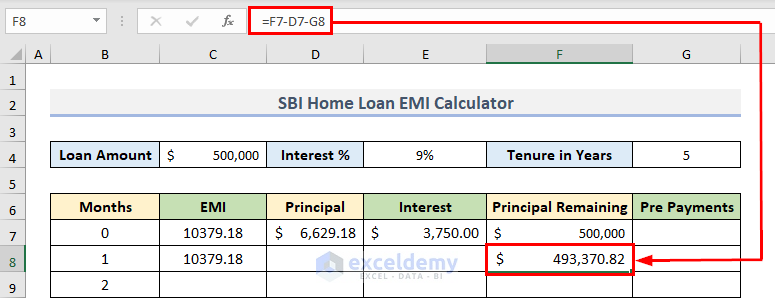
Here, we subtract the Pre-Payments and Principal from the Previous Remaining Principal to get the Remaining Principal Amount.
Step 6 – Use Fill Handle to Complete Dataset
- Select a cell with a formula and put the mouse cursor bottom right corner. The cursor will change into the plus (+) symbol, which is the Fill Handle icon.
- Drag the Fill Handle down to duplicate the formula over the range. Alternatively, double-click on the icon.

- Repeat the same process for the rest of all the columns to copy formulas.
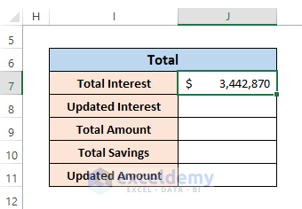
Step 7 – Update Total Interest and Amount
- Put the Total Interest which is in our case, $3,442,870.
- Choose cell J8 and copy this formula into that cell.
=SUMIF(E7:E67,">0")- Hit the Enter key to complete the process.
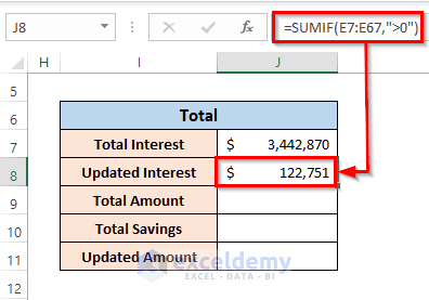
How Does the Formula Work?
The SUMIF function determines if a condition is true or false before adding the values in a range. When the result is larger than 0, this formula will provide results.
- Further, we utilize the formula using addition for computing the Total Amount.
- As a result, select cell J9 and put the addition formula into that cell.
=C4+J7- Press the Enter key to see the result of the total amount.
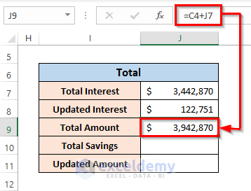
Here, by adding Loan Amount and Total Interest we can just get the Total Amount. To calculate the Total Savings, we are using the subtraction formula.
- Select cell J10 and use the formula:
=J7-J8- Press Enter.
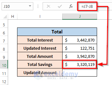
Here, by subtracting Updated Interest from Total Interest we can acquire the Total Savings.
- The final calculation for this step is the Updated Amount. Select cell J11 and insert the addition formula into that cell:
=C4+J8- Press the Enter key on your keyboard.
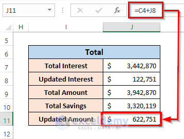
We add the Loan Amount and the Updated Interest we can obtain the Updated Amount.
Read More: Create Home Loan EMI Calculator in Excel Sheet with Prepayment Option
Step 8 – Use Prepayment Option to See Modifications
- Add prepayment (manually) in cells G10 and G12, and you will be able to see the changes in the whole row of those both cells.
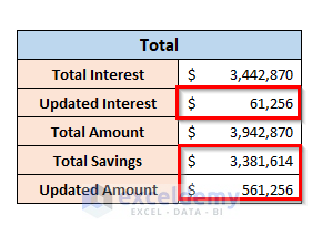
- You will notice changes in the Updated Interest, Total Savings, and Updated Amount after entering the prepayment value.
- As a consequence of the findings, we can conclude that after making the first prepayments, both the Total Savings and the Updated Interest decline.
Step 9 – Insert Chart for Better Visualization
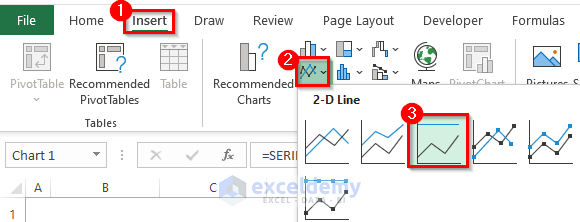
- Select the whole dataset and go to the Insert tab from the ribbon.
- In the Charts category, click on the Insert Line or Area Chart drop-down menu.
- Select 100% Stacked Line from the drop-down menu.
- A chart will appear on-screen.
- Click on Chart Filters and check mark EMI, Principal, and Interest.
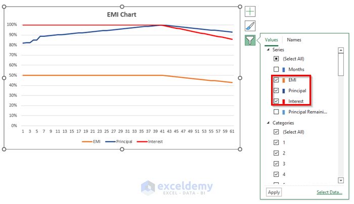
- Here’s a sample EMI Chart.
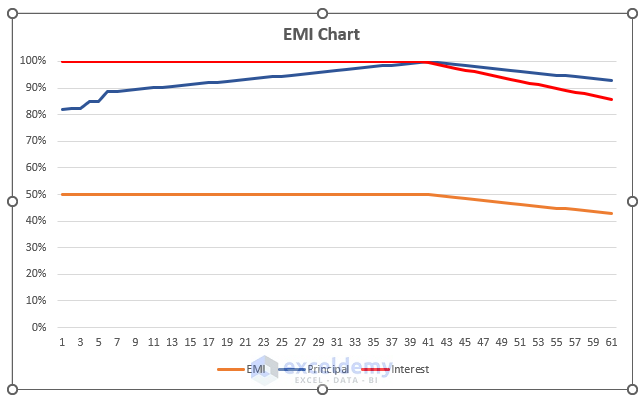
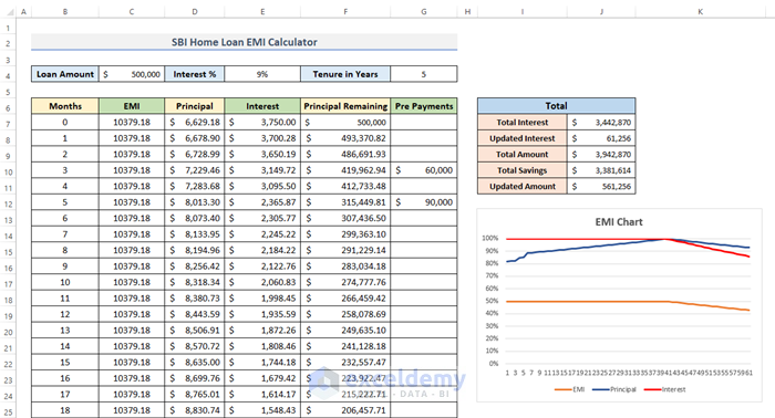
Final Template
This is the final template of the SBI home loan EMI calculator in an Excel sheet with a prepayment option and a chart for visualizing the data.
Things to Keep in Mind
- If you enter a loan that lasts more than 5 years into the calculator above, you will need to add additional rows.
- The Interest Rate should be in the Percentage Number Format.
Download Template
You can download the Home Loan EMI calculator with the prepayment option and use the template for your work.
Related Articles
- Personal Loan EMI Calculator Excel Format
- Reducing Balance EMI Calculator in Excel Sheet
- How to Create Reverse EMI Calculator in Excel
<< Go Back to EMI Calculator | Finance Template | Excel Templates
Get FREE Advanced Excel Exercises with Solutions!

In this explaination you have directly entered Total Interest as 3442870. but you have not told how did you arrived to that amount. i am not able to understand what amount to be taken when i change the loan amout. will you please reply to my email id: [email protected]
will wait for your reply.
Hello Jagadeesh,
Thank you for your thoughtful question! The Total Interest (₹3,442,870) wasn’t entered manually — it’s calculated using this formula:
Total Interest = (EMI × Total Months) − Loan Amount
So, when you change your loan amount, interest rate, or tenure, Excel will automatically recalculate the total interest based on the new EMI. You can also confirm this by summing up the Interest column in the amortization schedule.
Regards,
ExcelDemy