Create Home Loan EMI Calculator in Excel Sheet with Prepayment Option

What Is Home Loan EMI?

EMI stands for Equated Monthly Installment, which is the amount of money that you need to pay monthly on a home loan. The formula for EMI is:

EMI=[PxRx(1+R)^N]/[(1+R)^N-1]

where,

P = Principal Amount
R = Rate of Interest
N = Repayment Periods (Total Number of Months)

So EMI depends on the interest rate (R), tenure years (how many years to repay the loan (N)), and also on your income.

The EMI has two main parts: Principal Amount and Interest Amount. The principal amount is less initially but increases with tenure, while the interest amount is high at the beginning and decreases over time. For this reason, it is recommended to try to make pre-payments during the initial months.

Home Loan Calculator with Prepayment Option: Create with Easy Steps

Step 1 – Create the Dataset for Home Loan EMI

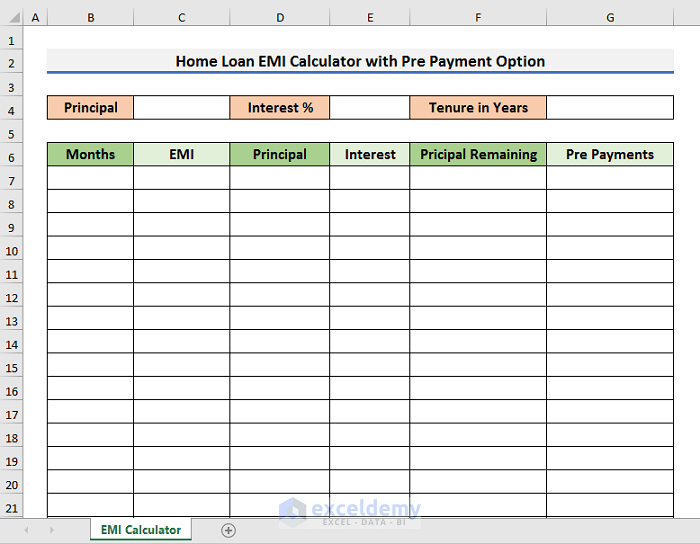
Create a dataset like the picture below, including sections for Principal, Interest %, and Tenure in Years.
Create columns for Months, EMI, Principal, Interest, Principal Remaining, and Pre-Payments.

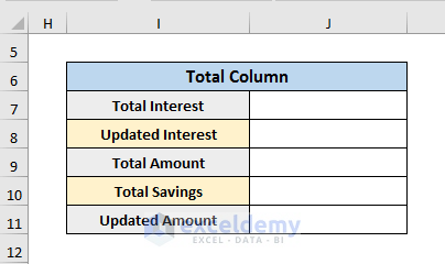
Create a section for all the total amounts including Total Interest, Updated Interest, Total Amount, Total Savings, and Updated Amount.

Step 2 – Insert Home Loan with Interest

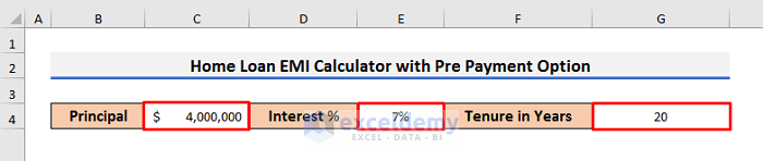
Enter the amount of the loan in Cell C4, the percentage of interest in Cell E4, and tenure in years in Cell G4.
In our case, the home loan is $4,000,000, interest is 7%, and tenure is 20 years.

Note: The Interest Rate should be in the Percentage Number Format.

Step 3 – Fill In Months and Principal Remaining Amount

Since 20 is the Tenure in Years, we need to enter 20*12 = 240 months in the Months column, starting from 0.

Select Cell B7 and type 0.
Drag the Fill Handle down to Cell B246.

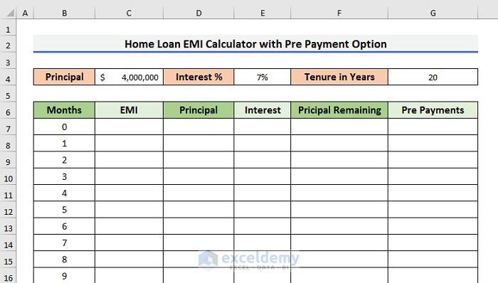
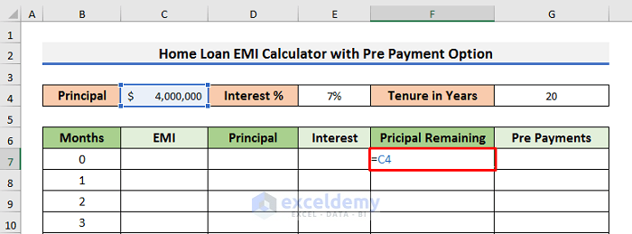
Select Cell F7 and enter:

=C4

Press Enter to see the result.

The value of Cell C4 is displayed, which is $4,000,000.

Step 4 – Apply Necessary Formulas in Dataset

With the required data in place, we can now apply the necessary formulas in the dataset, starting with the EMI formula.

In Cell C7 enter the formula below:

=ABS(PMT(E4/12,G4*12-B7,F7))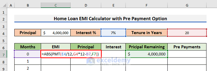

In this formula, we use the PMT function to calculate the EMI, and obtain the absolute value of this result with the ABS function.

The first argument (E4/12) is the Monthly Interest Rate.
The second argument (G4*12-B7) denotes the Number of Months Remaining.
The third argument (F7) represents the Remaining Principal Amount.

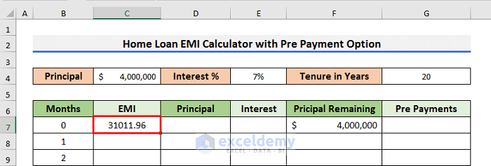
Press Enter to see the result.

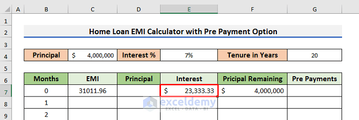
In Cell E7 enter the formula for the Interest amount:

=$E$4/12*F7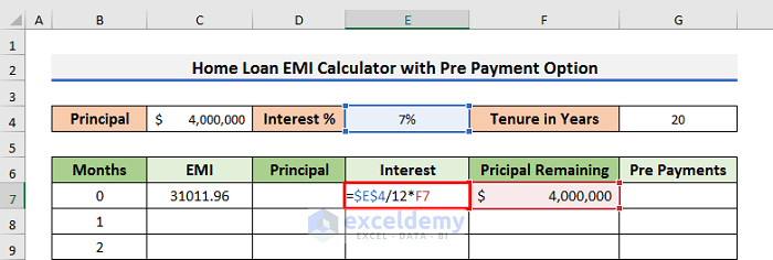

In this formula, we divide the Yearly Interest Rate by 12 to get the Monthly Interest Rate, then mutiply it by the Remaining Principal Amount to get the Interest Amount.

Press Enter to see the result.

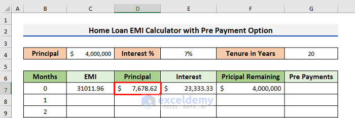
To find the Principal amount, enter the below formula in Cell D7:

=C7-E7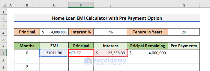

Press Enter to see the result.

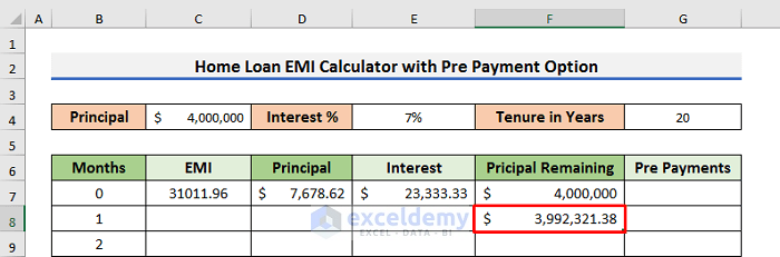
To calculate the Principal Remaining, enter the below formula in Cell F8:

=F7-D7-G8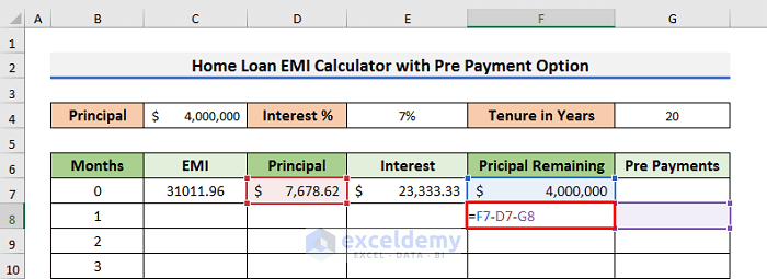

To get the Remaining Principal Amount, we subtract the Pre-Payments and Paid Principal from the Previous Remaining Principal.

Press Enter to see the result.

The EMI will be fixed for the rest of the months.

Enter the formula below in Cell C8:

=$C$7

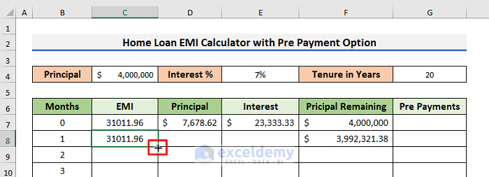
Step 5 – Use Fill Handle to Complete Dataset

After inserting the formulas, we apply them to the whole sheet.

Select Cell C8 and put the cursor on the bottom right side of the cell.

The cursor will change into a small black plus (+) sign, called the Fill Handle.

Double-click on the Fill Handle sign or drag it down to Cell C246.

Repeat the same procedure for the rest of the formulas.

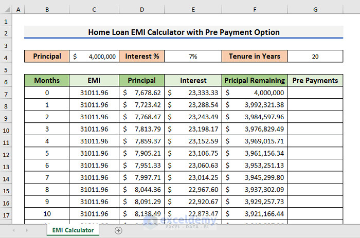
Optionally, we can add freeze panes to see all the rows while retaining the headers:

Select Cell B7.
Go to the View tab and select the Freeze Panes icon.

The result is like the picture below. We can scroll down to the bottom without losing sight of the headers.

Step 6 – Update Total Amount and Interest in Dataset

Now we can apply formulas to update the Total Amount and Interest in the dataset, starting with the Updated Interest.

In Cell J8 enter the formula:

=SUMIF(E7:E246,">0")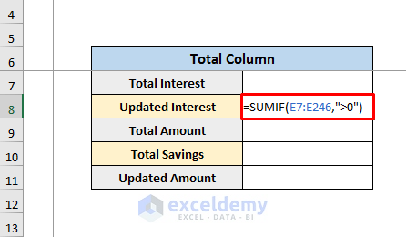

In this formula, we use the SUMIF function to calculate the Updated Interest amount. This formula will show results when the result is greater than 0.

Press Enter to see the result.

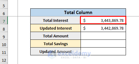
Enter the value of the Updated Interest in Cell J7.

Select Cell J9 and enter the formula:

=C4+J7

This denotes the Total Amount.

For Total Savings, enter the below formula in Cell J10:

=J7-J8

For Updated Amount, enter the below formula in Cell J11:

=C4+J8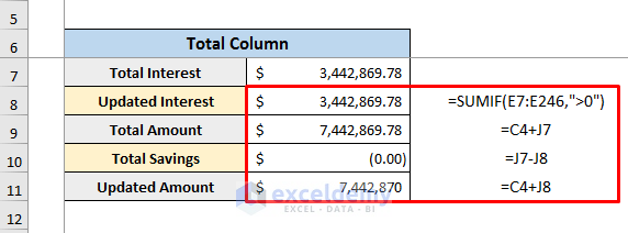

Step 7 – Use Prepayment Option to See Changes

Add prepayments in Cell G10 and G12.

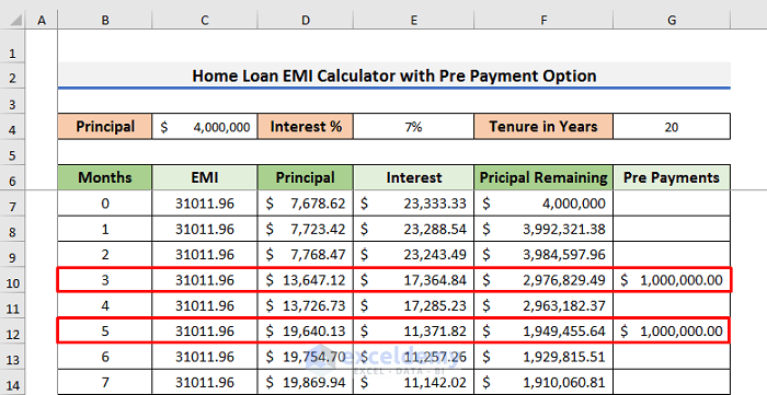
After entering the pre-payments value, the changes appear in the Updated Interest, Total Savings, and Updated Amount.

From the results, we can say that after making prepayments in the initial months, the Total Savings increase, and the Updated Interest decreases.

Things to Remember

In the above calculator, if you add tenure years of more than 20 years, then you need to create more Rows to accommodate the extra values.
When you are calculating the EMI, be precise with the arguments inside the formula.

Download Practice Calculator

Home Loan EMI Calculator with Prepayment Option.xlsx

<< Go Back to EMI Calculator | Finance Template | Excel Templates

Get FREE Advanced Excel Exercises with Solutions!

6 Comments

Abu Jul 1, 2022 at 10:54 AM

Thank you very much for sharing this,

could you share, how to print the expected end date dynamically after each part payment.
- Reply
  Mursalin Jul 19, 2022 at 4:52 PM
  
  Hello, Abu!
  Thanks for your comment. Unfortunately, it is not possible to show the expected end date dynamically after each pre-payment. Because the dataset changes dynamically after a pre-payment. But you can find the expected payment date after each month using the formula below. For the dataset, we have used in this article, you can type the formula in Cell H8:
  =DATE(YEAR(H7),MONTH(H7)+(12/$J$15),DAY(H7))
  Here, Cell H7 contains the loan starting date and Cell J15 contains the number of yearly payments.
  You can also take a look at this article https://www.exceldemy.com/student-loan-payoff-calculator-with-amortization-table-excel/ for an explanation of the formula. I hope this will help you to solve your problem.
  Thanks!
tanveer Nov 16, 2023 at 3:24 PM

hello,
thank you for sharing wonderful template.
can you please also help to add floating interest rate column, as maximum loans are in floating rates in India.
- Reply
  Tanjim Reza Nov 19, 2023 at 5:55 PM
  
  Hello, TANVIR!
  Thank you for your query. Regarding your query, to get a home loan emi calculator with floating interest rates, you will need a new mortgage calculator where interest rates vary.
  To help you, I can link you to another of our tutorials which exactly will serve your needs.
  https://www.exceldemy.com/loan-amortization-schedule-excel-with-variable-interest-rate/
  
  Please download the template from the above link and go through the article to learn how to use it. Hope, it will help.
  
  Regards,
  Md. Tanjim Reza Tanim
Dorababu Feb 6, 2024 at 9:21 PM

I thought like number of emi’s will be reduced when we pay the principal amount can I get that?
- Reply
  Lutfor Rahman Shimanto Feb 25, 2024 at 9:50 AM
  
  Dear DORABABU
  
  Thank you for your comment and your insightful observation. You are correct in pointing out that making prepayments towards the principal amount of a home loan can indeed result in a reduction in the total number of EMIs. This is an important consideration and can have a significant impact on the overall loan repayment timeline.
  
  To incorporate this feature into the home loan EMI calculator, you can make the following adjustments to the existing formula:
  
  Update Total Number of Months (N):
  
  Instead of fixing the total number of months as G4×12, you can dynamically adjust it based on the prepayments made. You can introduce a new variable, say M, representing the total number of months after considering prepayments. The formula for M would be: M=G4×12−Number of Prepayment Months
  
  Modify the PMT Function for EMI Calculation:
  
  Update the formula for EMI calculation (in cell C7) to reflect the adjusted total number of months (M): =ABS(PMT(E4/12,M,F7))
  
  By making these changes, the calculator will dynamically adjust the total number of EMIs based on the prepayments made, providing you with a more accurate representation of the impact of principal payments on the loan tenure.
  
  I hope this addresses your query. If you have any further questions or if there’s anything else you’d like to discuss, please feel free to ask.
  
  Best Regards
  
  Sumaiya Mirza
  
  ExcelDemy