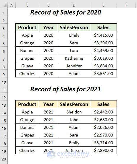
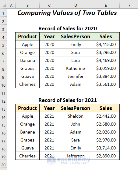
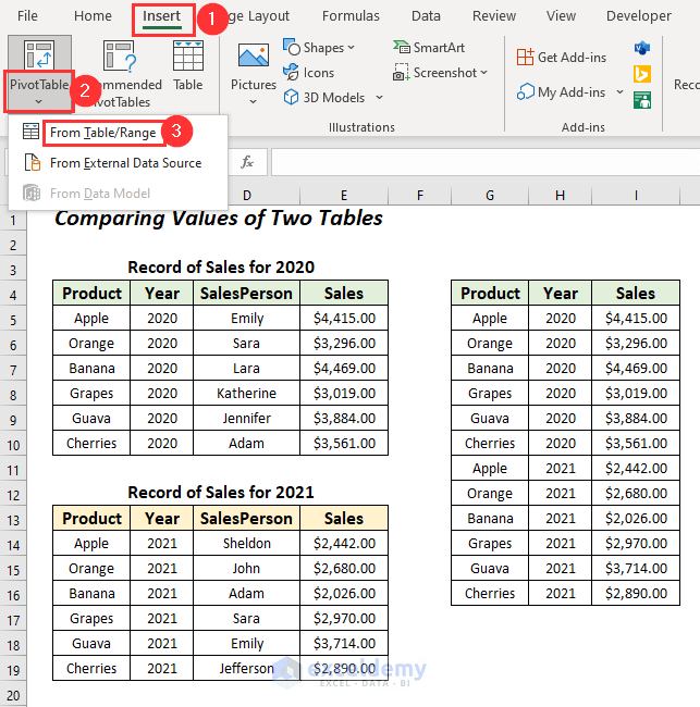
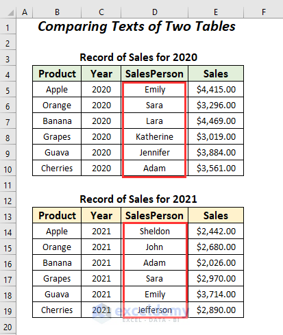
How to Compare Two Pivot Tables in Excel (3 Suitable Examples)

Here we have the following two datasets containing the sales records for 2020 and 2021 for different products of a company. In this article, we will try to compare these two tables either by values or text.

Example 1 – Using Formula to Compare Two Pivot Tables in Excel

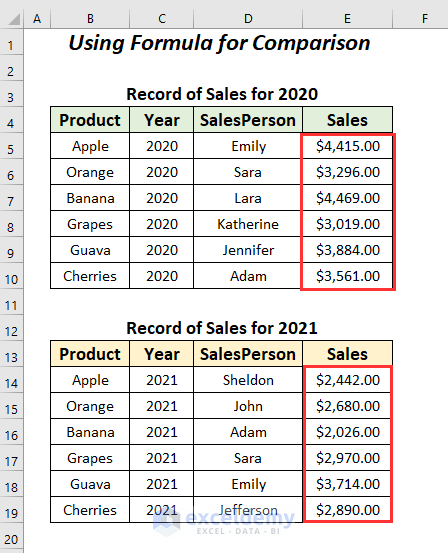
Here, we will use the GETPIVOTDATA function to calculate the differences between the sales values of different years.

Step 1 – Creating Two Pivot Tables in One Sheet

Go to the Insert tab, choose PivotTable dropdown, and pick From Table/Range.

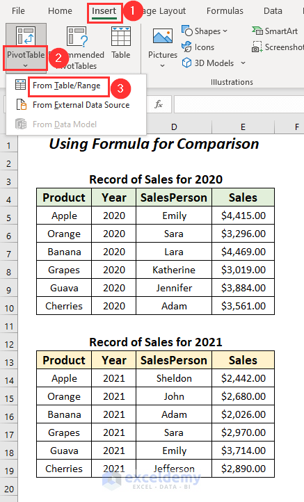
You will get the PivotTable from table or range dialog box.
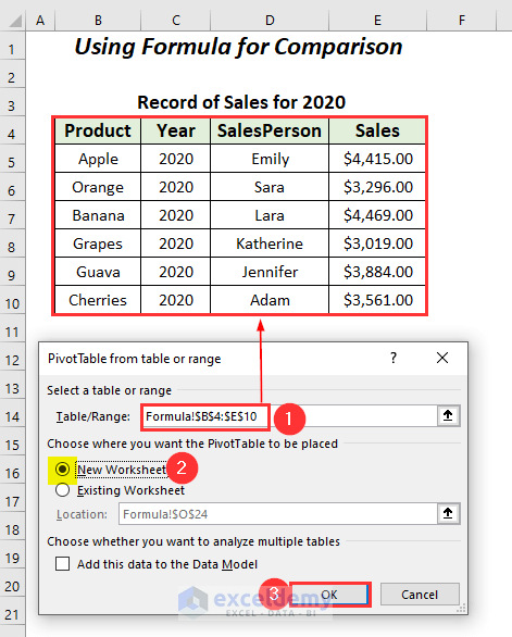
Select the range of the first table for the Year 2020 in Table/Range.
Click on the New Worksheet option and press OK.

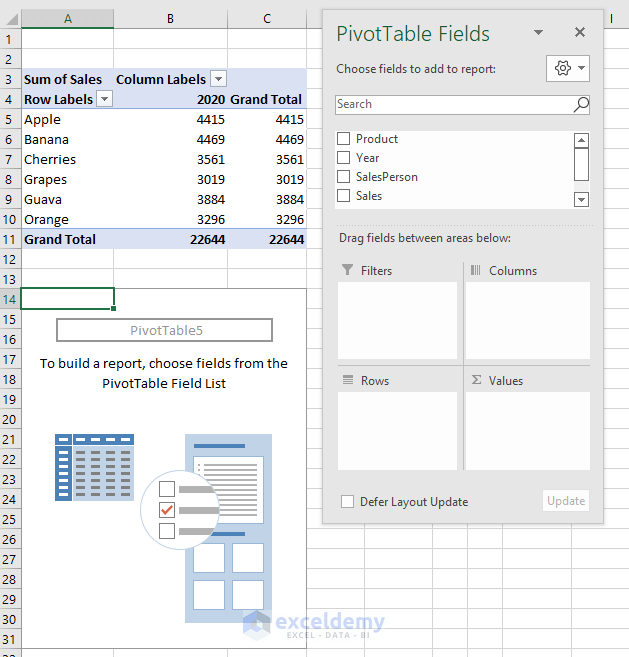
You will be taken to a new sheet where you will have two sections: PivotTable3 and PivotTable Fields.

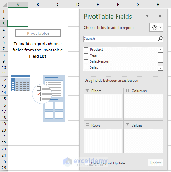
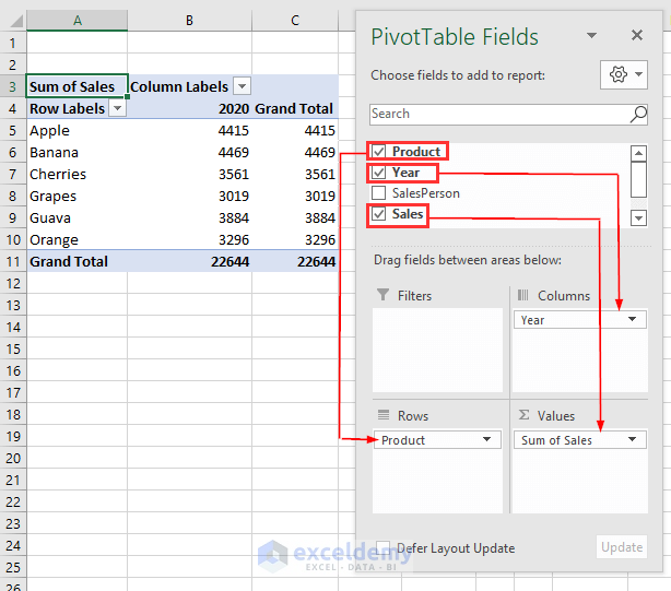
Drag down Product to the Rows area, Year to the Columns area, and Sales to the Values field.

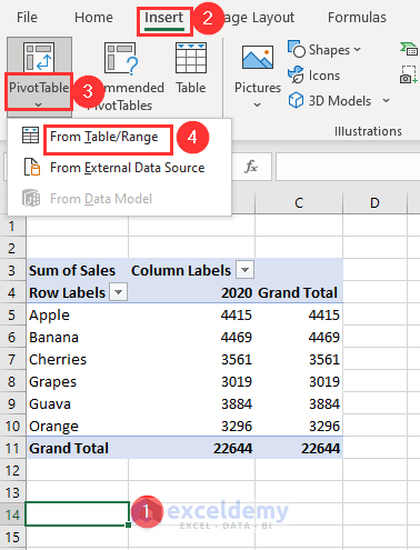
Click on cell A14 (or another cell that doesn’t contain parts of the previous pivot sheet), go to the Insert tab and choose From Table/Range for PivotTable again.

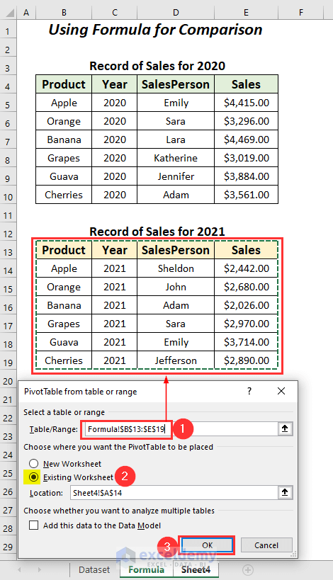
Select the range of the second table for the Year 2021 in the Table/Range
Click on the Existing Worksheet option and press OK.

You will get a new PivotTable and its related fields.

Drag down Product to the Rows area, Year to the Columns area, and Sales to the Values

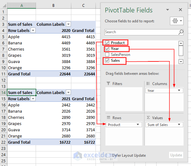
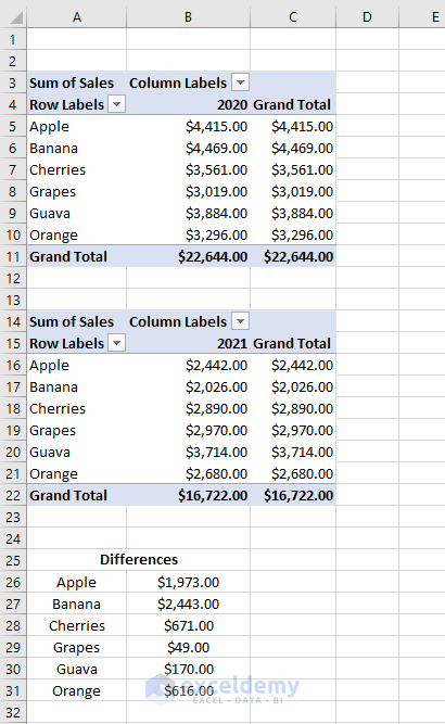
This inserts two pivot tables in one sheet and creates a space for displaying the differences for different products.

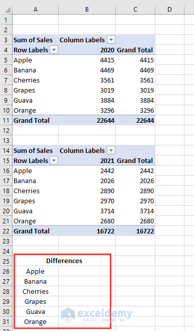
Step 2 – Insertion of Formula to Calculate Differences

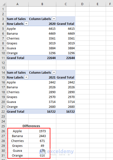
Copy the following formula in the cell B26:

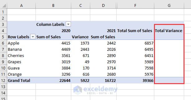
=GETPIVOTDATA("Sum of Sales",$A$5,"Product",A26)-GETPIVOTDATA("Sum of Sales",$A$16,"Product",A26)

Here, the Sum of Sales is the Field from which we want to get the values, $A$5 is a cell of the first PivotTable from which we want values, Product is the Field name, and A26 is the Item name of this Field. For the second portion, $A$16 is a cell of the second PivotTable from which we want values.

Formula Breakdown

GETPIVOTDATA(“Sum of Sales”,$A$5,”Product”,A26) → becomes
- GETPIVOTDATA(“Sum of Sales”,$A$5,”Product”, “Apple”)
  - Output → 4415
- GETPIVOTDATA(“Sum of Sales”,$A$16,”Product”,A26) → becomes
  - GETPIVOTDATA(“Sum of Sales”,$A$5,”Product”, “Apple”)
    - Output → 2442
  - GETPIVOTDATA(“Sum of Sales”,$A$5,”Product”,A26)-GETPIVOTDATA(“Sum of Sales”,$A$16,”Product”,A26) → becomes
    - 4415 – 2442
      - Output → 1973

Drag down the Fill Handle.

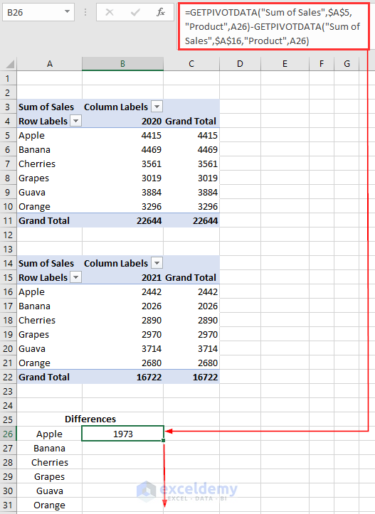
You will get the values for the rest of the cells.

You will be able to calculate all of the differences between the sales values for the years 2020 and 2021.

Example 2 – Comparing Values with Pivot Table by Combining Two Tables

Here, we will combine the following two datasets for the years 2020 and 2021 and then convert them into a PivotTable to show the differences.

Case 2.1 – Calculation of Difference Between Two Columns with Difference From

Steps:

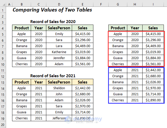
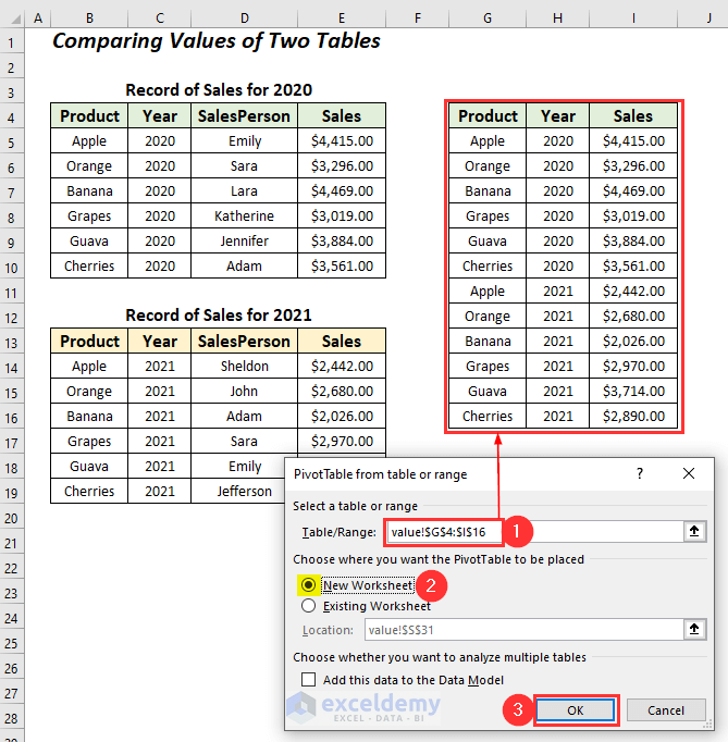
Combine the columns Product, Year, and Sales of the Years 2020 and 2021.

Go to the Insert tab, select the PivotTable dropdown, and pick From Table/Range.

You will get the PivotTable from table or range dialog box.
Select the entire range of the new table in the Table/Range.
Click on the New Worksheet option and press OK.

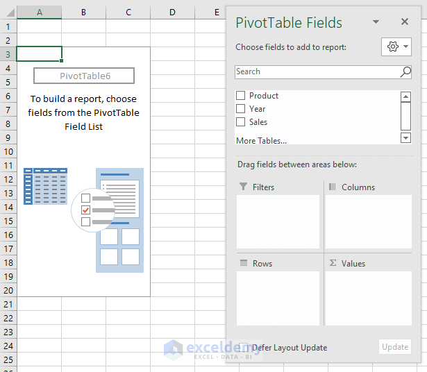
You will be taken to a new sheet where you will have two sections: PivotTable6, and PivotTable Fields.

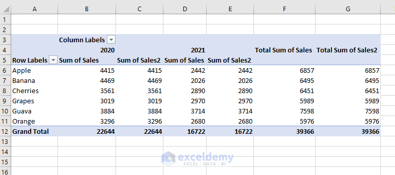
Drag down Product to the Rows area, Values to the Columns area, and Sales twice to the Values.

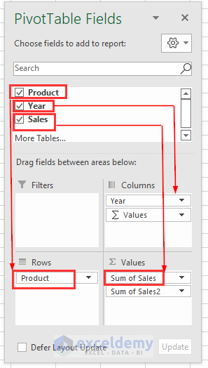
You will have Sum of Sales and Sum of Sales2 in the Values area.
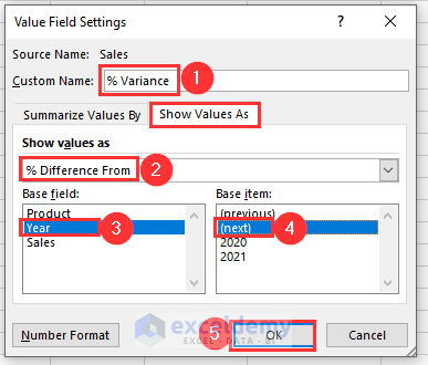
Click on the dropdown symbol of the Sum of Sales2 field and choose the Value Field Settings

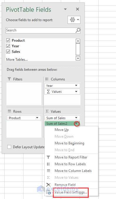
After that, you will get the Value Field Settings wizard.
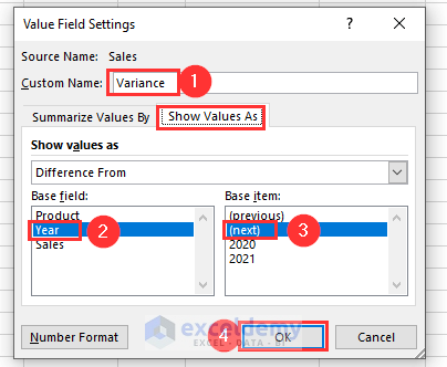
Set the Custom Name as Variance, go to the Show Values As tab and select the Difference From option, then choose Year as the Base field and next as the Base item.
Click on OK.

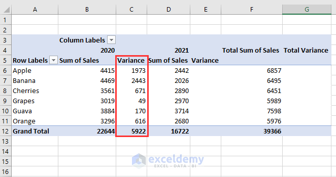
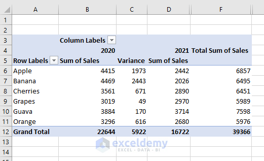
You will get the following Pivot Table where the first Variance column will contain the differences between the sales values for the years 2020 and 2021.
We also have extra columns named Variance and Total Variance where we don’t have values that we will hide.

Choose the Variance column and right-click.
Select the Hide option.

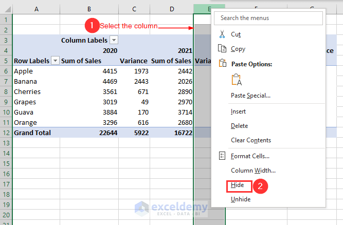
Repeat for the Total Variance column.

We now have the following pivot table with the differences in the sales values. Note that the Grand Total of Variance is summing the variances rather than displaying the difference in totals.

Case 2.2 – Calculation of Percentage Difference Between Two Columns

Here, we will calculate the differences in percentage form in the following table.

Steps:

Click on the dropdown symbol of the Sum of Sales2 field and choose the Value Field Settings

You will get the Value Field Settings wizard.
Set the Custom Name as % Variance, go to the Show Values As tab and select the % Difference From option, then choose Year as the Base field and next as the Base item.
Click on OK.

Then, you will get the following Pivot Table where in the first % Variance column you will get the differences between the sales values for the years 2020 and 2021.
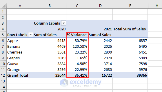
We have also extra columns named % Variance after 2021 and Total % Variance where we don’t have values that we will hide.

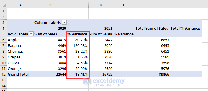
After hiding the second % Variance and Total % Variance we will get the following table with percentage differences in the sales values for the two years.

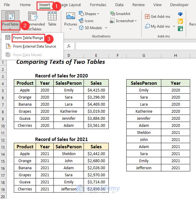
Example 3 – Comparing Texts with Pivot Table by Combining Two Tables

In this section, we will compare the Salesperson names for the two years 2020 and 2021.

Steps:

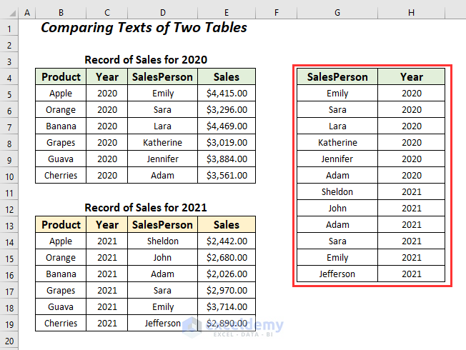
Combine the columns SalesPerson and Year of the two tables.

Go to the Insert tab, select the PivotTable dropdown, and choose From Table/Range.

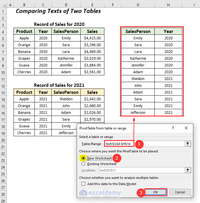
You will get the PivotTable from table or range dialog box.
Select the range of the new table in the Table/Range.
Click on the New Worksheet option and press OK.

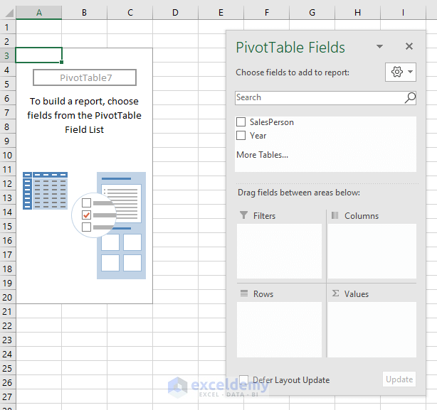
You will be taken to a new sheet where you will have two sections: PivotTable7, and PivotTable Fields.

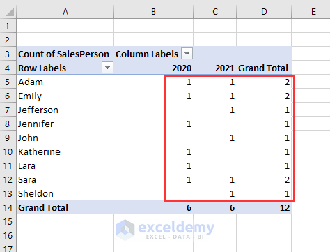
Drag down SalesPerson to the Rows area and Values area, Year to the Columns.

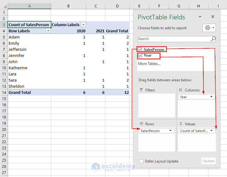
You will get the following table where you have the counting numbers under the year columns for different salespersons where 1 represents that this person works as a SalesPerson for that corresponding year.