Latest Posts From Rafiul Haq

To demonstrate our methods, we have a dataset with three columns: “Fruit,” “March Sale,” and “April Sale.” Method 1 - Using the FormulaR1C1 Property ...

In this method, we’re going to show you 6 ways for Excel VBA split string(s) into rows. To demonstrate our methods, we’ve chosen a dataset with 2 columns: ...
Method 1 - Changing Text Color to Hide Rows Based on Cell Value with Conditional Formatting Steps: Select the cell range B5:D10. From the Data tab ...

In this article, we’re going to show you 3 methods to convert multiple rows to columns in Excel Macro. For this purpose, we’ve taken a dataset with 3 rows: ...
We’ll use the following dataset, which contains four columns for employee attendance. How to Stack Rank Employees in Excel: 3 Easy Ways Method 1 - ...

.This sample dataset contains 3 columns: Quarter, Brand, and Share, regarding the global shipment of smartphones in the last quarter of 2021. Method 1 - ...
We'll use a simple dataset with item prices and percentage discounts to subtract them from the original price. Method 1 - Using a Percentage Formula ...
To demonstrate our methods to combine duplicate rows without losing data, we’ll use the following dataset: Method 1 - Merging UNIQUE, IF & ...

To demonstrate our methods, we’ll use the following dataset. Method 1 - Using Insert Link Feature Steps: Select cell B12. From the Insert ...

To demonstrate putting numbers in order, we’ll use a dataset with three columns: “No.”, “Name”, and “Car”. Method 1 - Using Context Menu to Put ...
Solution 1 - Gridlines Disappear in Excel If Those Are Turned off If Gridlines are turned off then the Gridlines will not be visible in Excel. To check ...

In this article, we’re going to show you 5 methods of how to use Excel to Filter a column based on another column. To demonstrate these methods, we’ve taken a ...
Method 1 - Utilizing Range.Offset Property in VBA Code to Find Duplicate Rows in Excel Steps: From the Developer tab >>> select Visual Basic. ...
We have two tables that show the pricing of the same product in two shops. We'll highlight the differences between the price columns. How to Compare ...

Method 1 - Employing VBA to Select Range from Active Cell to the Last Non-Blank Cell Steps: From the Developer tab >>> select Visual Basic. ...
See Our Reviews at


Hello Baijul, Thank you for your question. The Date column needs to be in ascending order. You’re adding an earlier date to the end of the data, that’s why the formula is not working.
You can sort the data or use the following formulas:
Cell C148: =LOOKUP(2,1/($C$140:$C$145>$C$147),$B$140:$B$145)
This returns Samantha
Cell C149: =LOOKUP(2,1/($C$140:$C$145>$C$147),$C$140:$C$145)
This returns November 25, 2022
If you want to return the price of the second matched value, you can use the following formula that returns the value $715.
=INDEX(FILTER(D58:D63,ISNUMBER(SEARCH(“Lap”,C58:C63))),2)
profit percentage = (selling price – cost price) / cost price. Our calculation is correct. Additionally, commission is not usually included in the profit calculation.
Question 6: You need to return the price of the Mobile Phone sold by Aaron. This question is similar to question 3. So, I have asked to use different formula to do so.
Now, 1 is used as a logical value to identify the matching records based on the conditions specified by the formula. This enables the INDEX function to retrieve the desired value from the given range.
(B79=B71:B76)*(C79=C71:C76) returns, {0;1;0;0;0;0}. So, when we put 1 inside the MATCH function, it will return the second value. Thus, we have obtained the value $429.
Hello, Lori. The file is working correctly on our end. I think you need to “Enable Editing” from the protected view feature of Excel.
Thank you for your question. Here is your Indian Format.
Greetings, Nat Troy. We don’t have a large enough dataset to test your problem. Please send us your file to [email protected]. So we can take a closer look at the issue.
Thank you, Calvin, for your query. I’m replying on behalf of ExcelDemy. You need to select the values of column A and then apply the conditional formatting to them. The condition will be similar to this image. Steps do the formatting is already mentioned in this article.
You can duplicate the months below the first month for multiple months’ data. Moreover, if you need to remove the values, you can just click the cell range and hit the Delete button. I have added the leave record format for four months in the following file. This can be found on the LeaveReord sheet.
Leave Record for User
Greetings Ethan. I’m sorry to see you’re missing a feature. You can submit feature requests to Microsoft via their website or community forums.
Hello Andrew, Your question is not clear to us. Can you send the Excel file to [email protected]? So, we can take a closer look at the issue.
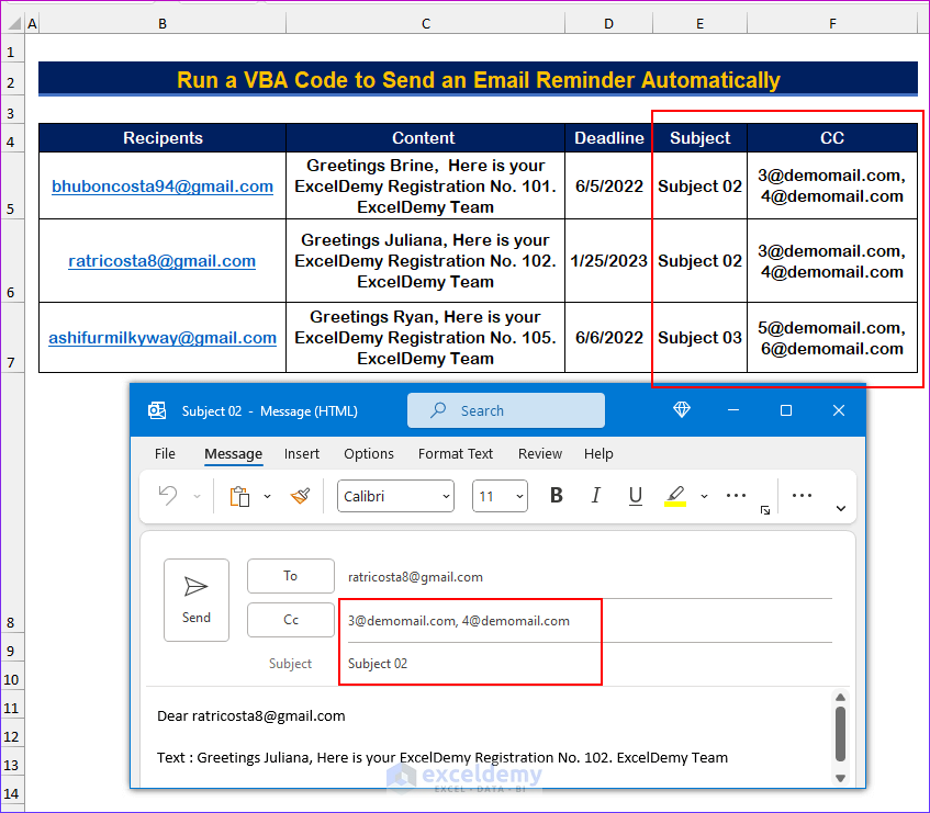
You can use the following code to include the subject and CC columns.
The following image shows the output.
Greetings, Fethiye Kiralik Villa. I am responding on behalf of ExcelDemy. I’ve tested the =hyperlink method, and it works perfectly for me. Make sure you have the latest version of Acrobat. Alternatively, you can try to reset all the settings in Adobe Acrobat Reader.
Greetings George. I am replying on behalf of ExcelDemy. There was an issue with the code in the file. I have updated the file. This works perfectly fine for a “+” character in the text.
Thank you, Alberto, for your question. I am replying on behalf of ExcelDemy. You can manually set the waiting time by using-
ActiveWorkbook.RefreshAll
Application.Wait (Now + TimeValue(“0:00:05”))
…..other lines of code
Here, it will wait for five seconds. You modify it to suit your needs.
Thank you, Gilles Laurence, for your comment. I am replying on behalf of ExcelDemy. The custom number format works perfectly on our end. The French number system uses a comma for a decimal separator and a space for thousand separators. You can change the thousand separators from the Advanced tab on the Excel Options to solve this.
Greetings, Michael. I’m responding on ExcelDemy’s behalf. Yes, the methods presented work the same way for Excel tables after I converted the provided dataset into a table.
Hi, Frank!
You can create a helper column and input “Yes” for the sent mails. Then, you can run the VBA code to sent the values without the “Yes” values. That way, the mail will be sent only to those not sent to before.
You can also email us your Excel file with detailed instructions to [email protected], so that we can give you a proper code to solve the problem.
Thank you, Rob, for your comment. To make the function available all the time, you can copy the code and paste the VBA code in a workbook. Then, save that workbook as Excel Add-in (*.xlam) file. Then, you will need to enable this add-in for a new Excel file. Thus, the function will be available as long as the add-in is enabled. Additionally, you will need to install the font beforehand.
Let’s assume, you have exported the Excel file as “code 128.xlam” file. Then, you will need to enable this (File > Options > Add-ins > select Go).
Then, you will need to enable the exported file name (in our case it is “code 128“) and press OK.
After doing this, whenever you create a new Excel file, you will be able to use this “CODE128()” function without copying the VBA code.
Hello, EG Barber thank you for your question. You can use the following code and paste inside your sheet (right click on the sheet, select View Code and paste the code there) to get an automatic VBA sum feature.
The following animated image shows the solution in action.
Hello Robin. This code should work for you. It will make the image fit in the output cell, keep the aspect ratio constant, and the image will not disappear.
Hello Danielle D, Thank you for your question. For the first question, you can add a line break using the CHAR function. CHAR(10) to be more specific. There are some feature limitations in the HYPERLINK method. You need to use the other methods to do more advanced stuff.
Then, for the second question, if you send your Excel file to [email protected], we will try to modify the VBA code according to your needs.
Hello Bill Allcock, Excel formulas can’t move data. So, we’re making a copy of the value. You need to use VBA to do so. Moreover, you can send us your sample Excel file to [email protected] and we will try to solve your problem using VBA.
Hello Andreas, you need to add the following line to ignore the error.
Thank you Anthony for your question. Let’s assume you have this data in 4 sheets and you want to copy the rows that has conflict.
Now, the output should contain only the “yes” from the 4 sheets:
To copy values from 4 sheets to a new sheet, use the following VBA code
Paul, we appreciate your analysis. That 1 represents column_number, which is an optional argument. You can omit that in the original formula and it will still return Ricky Ben.
=INDEX(B5:B24,MATCH(1,INDEX((C5:C24=100)*(D5:D24=100)*(E5:E24=100),0),0),1)
Thanks for your formula.
Just a reminder, if anyone wants to copy and paste this formula, the quotes need to be straight (“”), not curly (“”). Otherwise, they will get the #N/A error.
1. Excel 365
=FIND(MID(C5,LOOKUP(9^9,FIND(“/”,C5,SEQUENCE(LEN(C5)))),9^9),C5)
2. Earlier Versions
=FIND(MID(C5,LOOKUP(9^9,FIND(“/”,C6,ROW(1:100))),9^9),C5)
You can use this code to keep the image proportion.
Here is the output.
Hello Claudiu, thank you for your question. The following steps will execute the VBA code whenever you change the dates.
Press ALT+F11 to bring up the VBA window. Then, right click on “Sheet1” and select View Code.
Then, type the following VBA code. This code will call the SendReminderMail Sub whenever, a value changes in the cell range D5:D7.
Then, when you change the date, it will automatically execute the macro.
However, if this doesn’t solve your problem, you can mail us your Excel file with detailed instructions to: [email protected], and we’ll try to solve it as soon as possible.
Thank you, Dan, for your comment. If the values are in text format, then the COUNTIF function will return zero. You can see that we have used a IF formula, which returns TRUE when the value from column B is greater than five. Notice the output is in text format.
However, if this doesn’t solve your problem, you can mail us your Excel file to: [email protected], and we’ll try to solve it as soon as possible.
Hello Cielo. Thank you for your question. I have tested the function on Excel 365, 2021, and 2013 versions. On first two version, you simply press ENTER and the formula will be spilled. However, in Excel 2013 if you press that, it will only show the first value.
Here, we have typed the formula in cell C5.
Then, pressed CTRL+SHIFT+ENTER. But, only the first value is seen.
To solve this, you need to follow these steps:
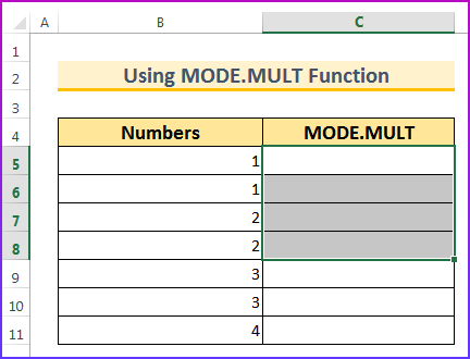
1. Select the cell ranges C5:C8 first.
2. Type the formula =MODE.MULT(B5:B11)
3. Press CTRL+SHIFT+ENTER. So, it will show all the mode values. Additionally, we have selected four cells, but there are only three outputs. Therefore, there is a “#N/A” for that reason.
Hello Andrew, you can download this Excel file which allows users to enter any amounts (including zero payments). Here, you need to input your value in Total Periods cell.
you can download this Excel file which allows users to enter any amounts (including zero payments). Moreover, you can see amount to be paid at the last balance, which is 11,368.
Hello Kenneth Mayfield. you can download this Excel file which allows users to enter any amounts (including zero payments).
Hello, Michael Cooper. you can download this Excel file which allows users to enter any amounts (including zero payments).
We are glad that this article helped you.
Hello Gerry Candeloro, this works perfectly on our end.
Here the interest is compounded annually, and the payment due is Monthly and Bi Weekly.
Hey Buck, you can follow this article for no compounding interest.
Hi Sohel! Your problem is not clear to us. You can email us the problem [email protected]
Hello Elizabeth D Jones, the template was available on the top of the article. If you still cannot find the link, you can download from here.
You can split the payment schedule into desired quarters and calculate the payments using that quarters’ interest rates.
Different credit cards have different grace periods. You can send us your Excel file and we will look into it.
Hello Ravneet, you can follow this article and adjust your payments on the “Extra Payment” column.
Hi Lisa. You can use the YEARFRAC function to calculate the days difference in fraction of that year. Then, you can multiply the result with the annual interest payment (in this case, scheduled monthly payment*12) to include the pro-rata interest.
I have modified the VBA code from the second method to handle blank cells for your dataset. Please check the solution to your first comment.
Hello Amilia. Thank you for your question. You can use the following VBA code to ignore blank cells within the range.
Hello Missy, If you change the list it will change the results, both are the same. Your question “can I then edit the column with the book title in it?” is not clear to us. It will be better for us, if you create a sample Excel file of what you want and share it with us. Thanks.
Hi, you can learn about how to hide source data from this article.
Thank you Lyn for your comment.
You can try the ZIP method to remove password from the Excel file.
This may not work with Excel 365 version and you will need to use an “Excel password recovery utility”.
Thank you Chelsea for your comment. We have checked the code and it’s working perfectly on our end. Here, we have set the date as
and 1 as the increment.
Did you follow the steps correctly? If yes, then you can send your Excel file and we can take a look into that.
Thank you Brian for your comment.
Actually, we believe you are right. However, in Excel the NORMDIST function shows the probability mass function when it is set to False. We have kept the original naming as it.
Moreover, if you go through the official documentation, you will notice it is written as “density function” in the latter part. So, chances are it may be displayed as ”probability mass function” but actually it is calculating the ”continuous values”.
You can do that by following these three steps:
1. You can insert any files using the Insert > Object command.
2. Save as PDF and Email Attachment.
3. Apply this code on a VBA Button.
Hey Ash, thank you for your question.
Suppose, we have these three items in cell Z2 as a Dropdown List:
X
Y
Z
Then, if we choose X, then it should display as a list in AA2 cell:
P
Q
R
Now, to do that, select cell range that contains PQR (eg. T1:T3), then use Name Range
PQR as X. Similarly, name the ranges as Y and Z for their corresponding cell ranges.
Next, use Data Validation on cell AA2.
Allow: List
Source: =INDIRECT(Z2)
Then, it should do what you want.
TLDR; Use Name Range and INDIRECT function inside Data Validation.
Thank you MOE for your wonderful question. To do this you need to apply the following Custom Cell Format.
You can do this by combining IF function with your formula.
Create multiple tables for your price information for the years. Refer the year to a cell and the use it to change the VLOOKUP’s “table_array”.
For example the year is on cell F4,
now you can type, =IF(F4=2023,IFERROR(VLOOKUP(B5,’Material Pricing’!B5:D7,3,0),””),IF(F4=2024,IFERROR(VLOOKUP(B5,’Material Pricing’!B13:D15,3,0),””),””))
If the year is 2023, then the “table_array” will be B5:D7
IF 2024, it will be B13:D15.
Else it will return a blank.
To know more about this, you can read this.
Thank you for your reply, Thor.
Thank you for your question. You need to use Underscore (“_”) between two words in the Name Range.
Thank you for your question.
In my second code, instead of “ActiveSheet.Pictures.Insert” you can try using “ActiveSheet.Shapes.AddPicture”, which should embed the images in the Excel file and it will not disappear.
the modified VBA code from the second method will be:
You are welcome. I am glad that this article was useful to you.
You need to change Google Drive’s Shared URL when inputting it into the cell.
For example, if I share an image the URL will be -> “https://drive.google.com/file/d/18r34oAVY8-bicTmf3CaTIumuHp_hqZxH/view?usp=sharing”.
Then, I need to change it to -> “https://drive.google.com/uc?export=view&id=18r34oAVY8-bicTmf3CaTIumuHp_hqZxH” (putting the values after d/ inside the id values of the URL).
And for your second question, I think the URL is not correct, if I remove the image resolution info from the URL, then it works perfectly in my second code.
Your URL -> “https://www.exceleinfo.com/wp-content/uploads/2022/06/Referencias-3D-en-Excel-1024×477.png”.
it should be -> “https://www.exceleinfo.com/wp-content/uploads/2022/06/Referencias-3D-en-Excel.png”.
According to your example, Set cRange = Range(“C5, C8, C11”)
Then, you’ll need to change the height & width to MergeArea
.Width = cItem.MergeArea.Width
.Height = cItem.MergeArea.Height
Full Code >
The output will be this: https://ibb.co/KXHVzSC
Thank You.