Latest Posts From Naimul Hasan Arif
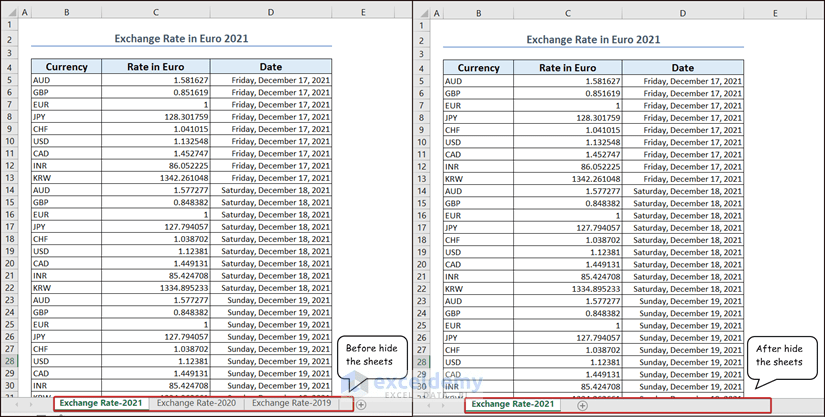
Sometimes, we might wonder to hide the secret or unnecessary sheets in terms of working with Excel. If you are looking for a better way to do it, you are ...

Advanced VLOOKUP in Excel: Knowledge Hub Use VLOOKUP for Multiple Columns VLOOKUP from Multiple Columns with Only One Return Use VLOOKUP to Return ...
This is the sample dataset. How to Launch the VBA Editor in Excel Go to the Developer tab and select Visual Basic. Click Insert and ...
![[Fixed!] Excel VBA Run Time Error 1004](https://www.exceldemy.com/wp-content/uploads/2023/05/5.-Use-Same-Name-in-Naming-Sheet-have-Excel-VBA-Run-Time-Error-1004.png?v=1697520324)
Excel VBA Run Time Error 1004 is a very common error in Microsoft Excel while working with Visual Basic for Applications (VBA) macros. Although it's a common ...

Method 1 - Using the Set Print Area Command to Change the Print Area in Excel Select your Print Area —> Page Layout Tab —> Print Area —> Set Print ...
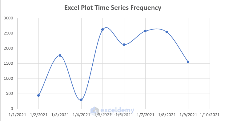
Are you looking for a better way to Plot Time Series Frequency in Excel? Well, I will try to explain two simple ways to plot time series frequency in Excel. I ...

Looking for ways to select a range with offset based on the active cell using VBA in Excel? Then, this is the right place for you. In order to select a ...

Looking for ways to sort named range using VBA in Excel? Then, this is the right place for you. In Microsoft Excel, a Named Range is a set of cells with ...

At the time of working with Microsoft Excel, we might face the necessity of disappearing MsgBox automatically. With the help of VBA, we can disappear MsgBox ...

In our day-to-day life, we need to deal with various bills. To organize the bill payment, we can create a bill payment checklist. In this article, I will ...

We like to have our data sorted. Sometimes, we might face the necessity to differentiate cells containing text from the entire dataset. In this article, I will ...

An Excel Event Calendar is a tool that tracks and schedules events, meetings, and appointments in a calendar format. It can be a useful tool for individuals ...
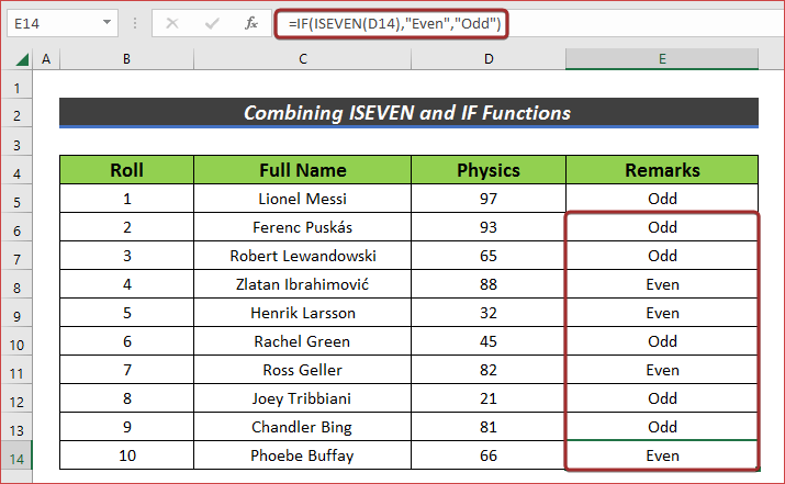
Verifying whether a number is odd or even can be a useful task in a variety of situations, such as data analysis or creating formulas for spreadsheets. In ...

Microsoft Excel is a powerful tool for organizing and analyzing data, but sometimes our data isn't always clean and error-free. That's where the IFERROR ...

Plotting a vector in Microsoft Excel allows you to visualize the data contained in the vector in the form of a graph or chart. This can be useful for seeing ...
- « Previous Page
- 1
- 2
- 3
- 4
- …
- 10
- Next Page »
See Our Reviews at


Hello MARIA, thanks for the comment and sorry for my late reply.
In the LOOKUP function, the first argument is Lookup_value. I have typed 2 just to signify the NUMBER format. You can type any number. It will work just fine.
Thanks all of you guys for your comments.
I think so many people are facing the same problem of applying the code in a range of cells. In our article, the VBA code that we have shown only works for a fixed cell. So, I am going to give you guys a slightly modified VBA code that will work for a range of cells( i.e. entire D column).
Private Sub Worksheet_Change(ByVal Target As Range)
Dim Oldvalue As String
Dim Newvalue As String
Dim mn As Range, pq As Range
On Error GoTo Exitsub
Set mn = Range(“D:D”)
For Each pq In mn
If Target.SpecialCells(xlCellTypeAllValidation) Is Nothing Then
GoTo Exitsub
Else: If Target.Value = “” Then GoTo Exitsub Else
Application.EnableEvents = False
Newvalue = Target.Value
Application.Undo
Oldvalue = Target.Value
If Oldvalue = “” Then
Target.Value = Newvalue
Else
Target.Value = Oldvalue & “, ” & Newvalue
End If
End If
Next pq
Application.EnableEvents = True
Exitsub:
Application.EnableEvents = True
End Sub
As the scale is different for each row, you can apply conditional formatting separately on each row with different colors. I hope that’s the simplest way to do so.
Hello AB,
Thanks for your response. We can certainly insert multiple photos in one row or column in a simple way. Just follow the following steps:
Select data > Home tab > Sort & Filter feature > Sort A to Z.
Thus, you will have all the images in a single column.
Similarly, you cam insert multiple photos in a single row.
Let me know if this is helpful for you or not.
Regards,
Naimul Hasan Arif
Hello CJ,
Thanks for your comment. To go into the details of your queries, let me break down the formula for you used in method 6 in a simpler form first.
The whole formula was:
=IFERROR(INDEX($D$5:$D$11, MATCH(ROWS($D$10:D10), COUNTIF($D$5:$D$11, “<=”&$D$5:$D$11), 0)), “”)
Here, the ROWS function counts the number of rows in the defined array.
ROWS($D$10:D10) → 1
The COUNTIF function compares the values in the given range and denotes them with a number based on the position in the smallest to largest order.
COUNTIF($D$5:$D$11, “<=”&$D$5:$D$11) → {4;6;1;5;2;3;7}
The MATCH function compares the values returned by the ROWS & COUNTIF functions and returns the index number of the position of the exact match.
MATCH(1, COUNTIF($D$5:$D$11, “<=”&$D$5:$D$11), 0))
MATCH(1, {4;6;1;5;2;3;7})→ 3
The INDEX function returns the third date value from the defined range in general form.
INDEX($D$5:$D$11, MATCH(ROWS($D$10:D10), COUNTIF($D$5:$D$11, “<=”&$D$5:$D$11), 0))
INDEX($D$5:$D$11, 3) → 43811
If there is an error in finding a date, the IFERROR function will return a blank cell as an output.
While applying the ROWS function, I have set a reference point from D10 and also finished the array on D10. That returns the number of row count 1. However, it is not mandatory that you have to set the reference point from D10. You can start from any cell between D5 to D11 but the starting and ending cell reference should be the same in that array. You can apply “ROWS($D$5:D5)” and it will return 1 too which is the same output.
If I am not wrong, the IFERROR function was introduced in the 2007 Excel version and the INDEX, MATCH, COUNTIF, & ROWS functions are available in the earliest Excel versions too. So, I hope it will work perfectly from the 2007 and the later Excel versions.
This formula can be applied to a dynamic table. It will automatically sort dates within the given range.
I hope you have the answers that you were looking for.
Regards,
Naimul Hasan Arif
Hello SAPTARSHI,
I have personally sent a mail with a mail body of more than 255 characters via the “Using VBA Macro to Automatically Send Email Using Outlook to Selected Recipients” method. The receiver got the mail with the full mail body. I have used Microsoft 365 and found no character restriction in this process.
Regards,
Naimul Hasan Arif
Hello MANESH KURKUTE,
Thanks for your response. Yes, we can certainly create the age bucket with negative numbers too. For this, just apply the following formula to have age 0 to -30 to the D-30 Days and -30 to -60 to the D-60 Days.
=IF(C5<= -30,”D-60 Days”,IF(C5<0,”D-30 Days”,IF(C5<=30,”1-30 Days”,IF(C5<=60,”31-60 Days”,IF(C5<=90,”61-90 Days”,”>90 Days”)))))
Regards,
NAIMUL HASAN ARIF
Exceldemy
Dear ROBERT STREMPKE,
Thanks for your comment. If you go through this article, you might have known that we can extract the defined information with the barcode through scanning. We can also have the sum of all goods in Excel. If you have multiple handheld readers, you can create a separate worksheet for each barcode scanner and summarize them in a new worksheet. In the summarized sheet, you can define the inventory stock balance and subtract the total sold products summing them from different sheets. I hope you have got what you are searching for.
Regards,
MD NAIMUL HASAN
Hello JAKE,
Thanks for your response.
The simplest way to highlight rows till a specific cell, instead of the entire row is to select the range till that column before applying the conditional formatting.
Then, you can apply any of the above methods and have your desired result.
If you have already applied the conditional formatting and want to change the selection range, go to the Home tab and click on Conditional Formatting. After that, select Manage Rules…
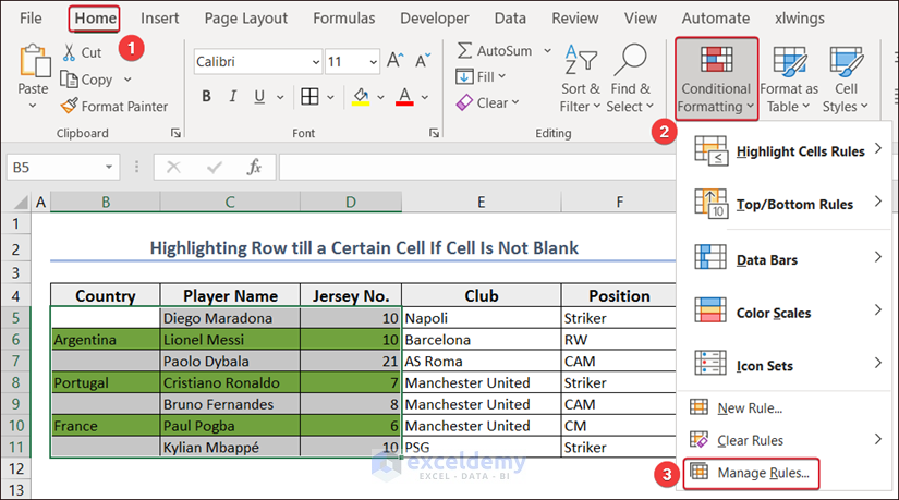
Now, change the range from the Applies to section and click on OK.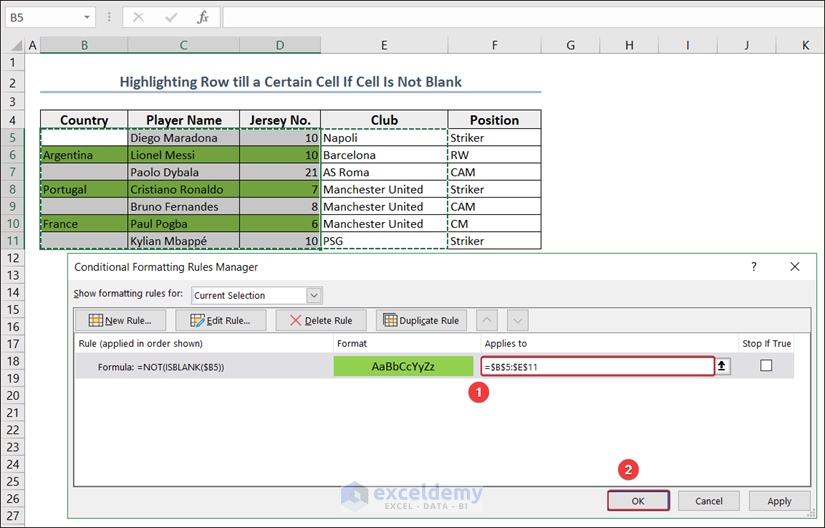
You will have the selection changed according to your desired cell.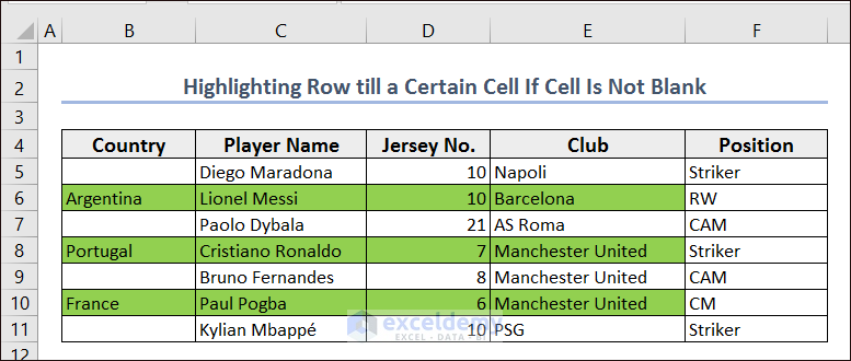
Dear G BHARATHI PRABHA,
Thanks for your response. I have used exactly the same code for my workbooks and it works perfectly. A little reminder for you that keep both the files in the same folder and keep both the files open. In order to avoid the error Subscript out of range, Try to run the code by keeping both the files open. I hope this will solve your problem.
Regards,
Naimul Hasan Arif
Dear GRAHAM,
I am using Office365 and I am getting my links retained from word to Excel. You can send us your file to have more clear solution.
Regards,
Naimul Hasan Arif
Dear TURAN,
Thanks for your valuable comment. That was an honest mistake from me. I have updated the error. I have also modified the code as I have found a simpler way to perform the same task.
Best Regards,
Naimul Hasan Arif
Dear CHARLES MOREHEAD,
Thanks for your valuable suggestion. I have considered the suggestion and updated the article.
Regards,
Naimul Hasan Arif
Hello JENELLE CASTRO,
Thanks for your question. If you have the same password in all the files placed in a certain folder, you can apply the following VBA code.
Make necessary adjustments in the code in the Path and Password sections. I hope this is the solution which you are looking for.
Regards,
Naimul Hasan Arif
Dear PA,
Thanks for your appreciation and valuable question. If you want to have 3 winners without repetition, you can follow the following procedure.
Create a column with random values using the following formula.
=RAND()
Then, apply the formula mentioned below in another column to rank the random values.
=RANK(D5,D5:D14)
Now, Insert the following formula where you want to have the winners’ names.
=XLOOKUP(C17:C19,E5:E14,C5:C14)
and press Enter to have multiple winners.
I hope this is what you are looking for.
Best regards,
Naimul Hasan Arif
Dear MUHAMMAD,
In order to apply the number to words conversion in all worksheets of a particular workbook., you can create a function and place it in a module. As you have created a function in a module, it will be available in all worksheets of that particular workbook.
Like I have created a module and a function named number_converting_into_words with the following VBA code.
Now, you can call the function in all worksheets of that particular workbook in the following way and have your number converted into words.
I hope you have found your desired answer.
Your regards,
Naimul Hasan Arif
Dear S. NARASIMHAN,
Thanks for your valuable comment. No, you do not need to pay any amount of dollars to have your question answered.
To clarify your query, I have considered a case where I have Product Name in B5:B9 but their sales value is in different columns in 3 different sheets. For sheet named January, the sales amount is in D5:D9 and for February & March sheets, the sales amounts are in E5:E9 & G5:G9. Followingly, I have applied the following formula to find the total sales value of iPhone.
=SUM(VLOOKUP(D12,$B$5:$D$9,{3},FALSE),VLOOKUP(B5,February!$B$5:$E$9,{4},FALSE),VLOOKUP(B5,March!$B$5:$G$9,{6},FALSE))Here, D12 refers to the product name which is to look for in the Product Name column, and return output from Sales to have the summation. As you can see in the formula, I have used {3}, {4}, and {6} to define the column having sales amount referring to the first column of the look-up range as 1.
I hope you have your desired output from the above discussion.
Your Regards,
Naimul Hasan Arif
Dear LUIS FERNANDO,
Thanks for the appreciation. Also big thanks to you for sharing your insights on the query of CHRISTOFER.
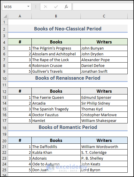
In response to your purpose, I have considered a case where I will have a drop-down with the names of the writers. Based on the writer selection, his books will appear in another drop-down just below the cell of the writer’s name.
I have assigned the following code in a button where I will have writers’ names without repetition under Uniquelist column. I have created a drop-down in cell C14 with those values. Similarly, I have sorted the matched books under Sorted Books column with the writer’s name in C14.
Now, select a writer name from drop-down and click on Sort button. You will have the related books’ name in the following drop-down and choose a book according to your preference.
Thanks a lot OSCAR APPELGREN for your questions.
In response to your first question to have matched rows entirely in the drop-down, it is not possible in Excel. A standard drop-down list in Excel does not support multiple rows of data.
If you want to filter multiple rows based on single or multiple criteria, you better use the FILTER function. It is not applicable to the older Excel version. It helps you to extract multiple matched rows quite easily than INDEX-MATCH functions.
According to your requirements to extract matched rows based on single criteria (i.e. year 2025), I have used the following formula which works pretty well.
=FILTER(B3:E17,D3:D17=H4)
And, for sorting rows with multiple criteria, you just need to use the asterisk sign(*) and insert the other condition.
=FILTER(B3:E17,(D3:D17=H4)*(E3:E17=H5))
Thanks a lot BABALOLA for the appreciation. It means a lot.
In response to your first question, let me break down the whole formula with IFERROR, INDEX, MATCH & SUM and explain it to you.
The first part of the formula here is IFERROR(INDEX(Jan!AH$9:AH$13,MATCH($B10,Jan!$B$9:$B$13,0)),0)
First of all the MATCH function looks through the value in range B9:B13 of Jan sheet whether it matches the value in cell B10. If it gets matched, it will return the related value according to the index from the AH9:AH13 range. The IFERROR Function is used to return a value(i.e. 0) if it can not find any proper value to return.
Similarly, I have gone through all 12 months’ sheets and added them with the SUM function.
In response to your second question, the & sign is used to concatenate cell AH$8 with the letter H. As it is considered a half match, 0.5 is multiplied. We have considered two half-matches to have the full match count.
Thank you PETE BAGALAYOS for your comment.
Yes, the change persists. Once you convert a variable from string to long, it remains in the long format. Well, if you need the string format, you will have to convert it from long to string again.
Dear SRECKO SELENDIC,
Thanks for your appreciation. It means a lot. In order to set sheet names based on cell reference, we can use a For loop along with Worksheets.name property. Here, I have written a code to split sheet and rename sheet split sheet keeping the main sheet name unchanged. Follow the following code to do so.
The output will be like the following image.
Dear JEFF,
Thanks for your comment. Here, the first method not only makes Excel full-screen but also hides the title bar along with tabs and ribbons.
The other methods also make Excel full-screen along with hiding tabs and ribbons but can’t manage to hide the title bar.
Hello Mark,
Glad to hear from you. There might be one of several reasons for not having the desired output. If the file is corrupted, protected, or scanned, there will be problem in extracting data. It will be helpful for me to specify the problem if you could send me the file and the code at [email protected].
Hello QUAN,
Thanks for your question. Here, {2,3} defines the cell number of the defined range B5:D10. 2 defines the row number and 3 defines the column number. Setting B5 as the base point and moving two rows and three columns, we will have the D6 cell which is expressed here with {2,3}.
Thanks for your appreciation. It means a lot.
To solve your problem, I will suggest you to change your separator from Control Panel. I hope it’ll solve the separator problem.
Thank you very much CHARLES DARWALL for your comment. The replies to your 2 problems is mentioned below:
In my case, the VBA works quite fine. Here, I have Kentucky as the last member in the States List column which is also the last member in the drop-down in cell B13.
Now, I have removed Kentucky as the last value in the States List column. So, Nevada is now the last value in the States List column which is also the last value in the drop-down.
After that, I have added Washington D.C. as the latest last member which has also been updated automatically in cell B12.
On the topic of your second question about being able to add a state in row 15 even if C is empty is because I have selected the range B5:B15 to add the drop-down list with the values in States List.
Hello BHAVNESH,
Have a look at Article 1 and Article 2. I hope it will help you to meet your desire.
In general, a new row is inserted above the selected cell when we use the insert command in VBA. In order to insert a new row/line, we need to modify the code. You can use the following code to do so.
Thanks for your response.
Normally additional information associated with Barcode is connected through a centralized dataset. When a UPC (Universal Product Code) code is scanned, the scanner sends the code to a server, which looks up the corresponding information in the database and sends it back to the scanner. In other cases like QR codes, the additional information might not be stored in a centralized dataset. QR codes can encode a URL that will take you to the related information regarding the product through scanning.
Thank you CARLOS for your concern.
As far as I am concerned I have followed the proper calculation process. There is an output difference between the arithmetic mean and the value using GEOMEAN. That’s the reason I think for the variation between the results. For further queries, you can contact [email protected].
Hello VULSTA KUZENA,
Thanks for your comment. In my case, the code runs just perfect. I have not got any error message. There might have some extra characters in that place. You can try it or send me the file to [email protected] to let me have a try.
Hello DAMON,
The process should work perfectly. It would be very helpful for me if you could just send me the file to give it a try.
Hello JACKIE,
Thanks for your comment. If we use these formulae, it will generate the date from that device (PC/Laptop/Mobile). So, check the date of your device first.
I think it will solve your problem.
Thanks SARAH for your comment and appreciation.
You can use the following VBA code with necessary changes to apply your code.
Sub AddRowFromAnotherSheet()
Sheets(“sheet1”).Range(“B7:E7”).Copy Sheets(“sheet3”).Range(“B9:E9”)
End Sub
Hello Darko,
Thanks for your valuable comment. This problem should not occur if the values are generated within Excel. However, This problem might happen if you copy and paste data from the web pages. In that case, there might have some non-printable characters which are preventing you from sorting data.
To check if there are any non-printable characters, use the LEN function to have the length of those cells.
If they are not giving proper output, apply the following formula to remove the non-printable characters.
=CLEAN(A1)*1
After that, I hope the Sort function will work perfectly.
If you look at our method 5, we have tried to apply conditional formatting based on a certain condition. The value was fixed all along the applied range.
Definitely possible. You just need to follow the following procedures to do so.
After selecting the entire dataset, go to the Insert tab. Followingly, click on Filled Map from the Maps option and you will have your desired output.
I will be glad if I could help you even a little.
The most important think here is to be careful about the code range. Input the range in the code according to your dataset.
For more simplification, you can try the following code where the code runs in range B3:B12 and sorts the values in the Ascending order.
Private Sub AutoSort(ByVal Target As Range)
If Not Intersect(Target, Range(“B:B”)) Is Nothing Then
Range(“B3:B12”).Sort Key1:=Range(“B3”), Order1:=xlAscending, Header:=xlNo
End If
End Sub
I hope it’ll run perfectly.
Thanks for your valuable comment.
A few factors might play a vital role in your problem.
1. As the file contains VBA code, the file must be saved in “.xlsm” format.
2. Don’t forget to change the ranges in your code. I have applied the code in D column. So, it’ll only be applicable in the D column.
Hi ISE. Thanks for your comment. Actually the date format is defined from the Number format. You can choose your date format from Number Format under the Home tab. There is no need to add VBA code to define date format.
Thank you AHAMED for your query.
For the explanation on how to mail merge Excel to Excel, you can check the following link:
https://www.exceldemy.com/mail-merge-from-excel-to-excel/
I hope it will fulfill your need.
Thanks for your appreciation. The solutions mentioned here should work perfectly. It would be helpful for us if you could kindly send the template. It would let us give a try.
Thanks for your comment. Look, I have used the following formula to Find If A Range of Cells Contains Specific Text in Excel.
=COUNTIF(B5:B19,”*”&D5&”*”)>0
Here, I have just mentioned the range B5:B19. So, in this way, it is not mandatory to know the exact row where Winter is Coming is written.
Thanks XAVIER for your correction.
Actually, there is just a little mistake in the code. Instead of writing B5:B, it’s been written B5:B10. This correction has worked perfectly for me.
You can submit more problems to us at [email protected]. Regards!
Thanks for your query.
It’s kind of a complicated task to filter specific data from certain cells of different worksheets with certain condition. I have tried a possible simple solution to pull data from different sheets into one sheet using FILTER function.I have used the following dataset for filtering the rows having Geller as Last Name and replace the Geller word with blank.
I have used the following formula to fulfill the purpose.
=FILTER(IF(Dataset!B4:J17=”Geller”,””,Dataset!B4:J17),Dataset!C4:C17=”Geller”)
For further information related to Excel, you can send message via email. email id: [email protected]
According to your requirements, you wanted to display the last 3 months’ data by a graph. You can follow the following procedure where I have tried to give you a simple solution that will help you display the last 3months’ data by graphical representation..
Create a new column, input the following formula in the 1st cell of that column and AutoFill till the cell you need. This additional column will define with numerical value the last 3 rows containing data.
=IF(AND(D4>0,ISBLANK(D5)),1,IF(B5=1,2,IF(B5=2,3,””)))
Next, create a Pivot Table with Months as Filters, Last 3 Months as Axis, and Sum of Product 1, Sum of Product 2, and Sum of Product 3 as Values.
Now, choose your preferred graphical representation format to display the last 3 months’ data.
Note: Don’t forget to refresh the Pivot Table after inserting the new month’s data. Otherwise, the graph won’t get updated. Alternatively, you can use Auto Update Pivot Table to lessen your hustle.
Thanks for sharing your valuable thoughts.
You can apply a formula combining VALUE and RIGHT functions to get the last 4 digits.
For example- you can use the following formula to get the last 4 digits of cell C5.
=VALUE(RIGHT(C5,4))
After that, apply the COUNT function to count the number of cells in that column.
I hope you wil get what you are looking for.
There is social media connection link in the introduction section about author. You can send message there.
Thanks for the appreciation.
In my case, it works just fine. It is very tough for me to give a solution without analyzing your code related to the dataset. It would be helpful for me if you could provide me your code.
Use of “for loop” function is a very simple approach for this purpose. You can use the following code to merged the defined cells to 100 tabs. Based on your sheets, you just need to change the value of “i” in the code.
Option Explicit
Public Sub FitTheMergedCells()
Call MergedCellsAutoFit(Range(“B5:C6”))
Call MergedCellsAutoFit(Range(“B7:C8”))
Call MergedCellsAutoFit(Range(“B9:C11”))
Call MergedCellsAutoFit(Range(“B12:C12”))
End Sub
Public Sub MergedCellsAutoFit(gg As Range)
Dim aa As Integer
Dim bb As Integer
Dim cc As Single
Dim dd As Single
Dim ee As Single
Dim ff As Single
Dim i As Integer
For i = 1 To 100
With Sheets(“Sheet” & i)
cc = 0
For bb = 1 To gg.Columns.Count
cc = cc + .Cells(1, gg.Column + bb – 1).ColumnWidth
Next bb
cc = .Cells(1, gg.Column).ColumnWidth + .Cells(1, gg.Column + 1).ColumnWidth
gg.MergeCells = False
ee = Len(.Cells(gg.Row, gg.Column).Value)
dd = .Range(“ZZ1”).ColumnWidth
.Range(“ZZ1”) = Left(.Cells(gg.Row, gg.Column).Value, ee)
.Range(“ZZ1”).WrapText = True
.Columns(“ZZ”).ColumnWidth = cc
.Rows(“1”).EntireRow.AutoFit
ff = .Rows(“1”).RowHeight / gg.Rows.Count
.Rows(CStr(gg.Row) & “:” & CStr(gg.Row + gg.Rows.Count – 1)).RowHeight = ff
gg.MergeCells = True
gg.WrapText = True
.Range(“ZZ1”).ClearContents
.Range(“ZZ1”).ColumnWidth = dd
End With
Next i
End Sub
Thanks for your appreciation and for sharing your modified code.
Yeah. There are ways to sort columns in descending order.
You can apply the following VBA in the dataset used in the first method to sort the data in descending order.
Sub SortSingleColumnWithoutHeader()
Range(“B5”, Range(“B5”).End(xlDown)).Sort Key1:=Range(“B5”), Order1:=xlDescending, Header:=xlNo
End Sub
Thanks ANDREW for your query.
You can check out the following formula that I have applied with the dataset mentioned in the image.
=INDEX(B5:E12,MATCH($B$15,$D$5:$D$12,0),0)
It gives the entire row with the first matched value. But it will not give all the matched rows as output. You can modify the formula using any aggregate function like SMALL to get all the rows at one go.
I have tried the following VBA code for all the cells in D Column. I hope this is the thing you are looking for.
Private Sub Worksheet_Change(ByVal Target As Range)
Dim Oldvalue As String
Dim Newvalue As String
Dim mn As Range, pq As Range
On Error GoTo Exitsub
Set mn = Range(“D:D”)
For Each pq In mn
If Target.SpecialCells(xlCellTypeAllValidation) Is Nothing Then
GoTo Exitsub
Else: If Target.Value = “” Then GoTo Exitsub Else
Application.EnableEvents = False
Newvalue = Target.Value
Application.Undo
Oldvalue = Target.Value
If Oldvalue = “” Then
Target.Value = Newvalue
Else
Target.Value = Oldvalue & “, ” & Newvalue
End If
End If
Next pq
Application.EnableEvents = True
Exitsub:
Application.EnableEvents = True
End Sub
You can apply the INDEX – MATCH functions combination to find out whether the value is matching with “2 ” or not in row 23 and then, use the INDIRECT function to retrieve the matched value with the value in row 6.
Thanks for your appreciation. It means a lot.
Unfortunately for some strange reasons, the formulas with the INDEX function don’t behave properly while starting from any other row but row 1. But luckily you have some other alternatives like the FILTER function in case your dataset start from row6
I have the use the following formula for this case.
=TEXTJOIN(“, “,TRUE,IF(F5=$C$5:$C$15,$B$5:$B$15,””))
Thanks for your query.
Yes, it is possible to apply multiple criteria. Not sure how your data looks, but according to your query, I have tried to reorganize it as follows to categorize names by region based on Vehicle.
=INDEX(B5:B15,MATCH(1,(B18=$D$5:$D$15) * (C18=$C$5:$C$15),0))
Thanks for your insight and for trying something on your own.
I’m afraid in an ideal scenario once you’ve used data validation with list of items to be selected, you will encounter an error since Excel anticipates values from that list only not any free text.
You can use the Clear property of the cell. You need to apply Range(“__your cell__”).Clear to make the selection cleared.
You can wrap your code in a loop to iterate continuously across a column if you want to traverse it.
If you want to traverse through a column, you can wrap your code with loop which will continue throughout the column.
As far as I’ve understood you are wanting to get value with category criteria, where for different categories items under those categories will show up. I’ve tried to visualize that like the following.
you can get the Products with respect to the category by using the following formula
=IF(ROWS($F$5:F5)>$C$15,” “,INDEX($B$5:$B$12,AGGREGATE(15,6,(ROW($C$5:$C$12)-ROW($C$5)+1)/($C$5:$C$12=$E$5),ROWS($F$5:F5))))
The Count column is obtained using the COUNTIFS function. =COUNTIFS($C$5:$C$12,B15). Feel free to access the reply-workbook.
Hi,
For columns A:
From the Data tab, select Data Tools and pick Data Validation from there. This will open the Data validation feature. From there, mention the text length of minimum “1” to maximum “8”.
For column B, follow the same procedure. Just in the maximum section, input “10”.
Thanks for the appreciation.
For columns A & B:
From the Data tab, select Data Tools and pick Data Validation from there. This will open the Data validation feature. From there, mention the text length of minimum “1” to maximum “8”.
For column C, follow the same procedure. Just in the maximum section, input “10”.
You can try using SpecialCells(xlCellTypeVisible) property while setting the detailsLastRow object. SpecialCells(xlCellTypeVisible) will trigger Excel to consider visible cells only. I hope this edited VBA will help you to get your desired output.
In case of making some effective lookup, every input should be unique (unless you are in any particular case) to get the related information. If you have some similar names, let’s assume some Employee Names, then use other particulars as input like Employee ID. If you don’t have this type of unique number (ID) column you can create it quite easily, for assistance do check https://www.exceldemy.com/excel-auto-generate-number-sequence/, then apply the lookup. I hope this will solve your problem.
Sorry DIEGO for my late response.
There needs to make some changes in the formula in case of finding the second last non blank cell.
I have used the following formula using LOOKUP function in cells D5 to D15 that is the chemistry marks in the dataset to find the second last non-blank cell.
=LOOKUP(2,1/((D5:D15<>D15)*(D5:D15<>“”)),D5:D15)
My dataset is given below:
Second Last Non Blank Value
Name Physics Chemistry
Green 164 110 (D5)
Jack 185 165
Joey 178 132
Mark 183 137
Austin 165 112
Marvin 173 119
Mason 186 170
Mount 170
Martin 177 160
Freeman 164
Federer 163 111 (D15)
Second Last Non Blank Value 160
For me it worked perfectly. I hope it will work the same way for you too.