Latest Posts From Mrinmoy Roy

Method 1 - Using Multiple If Conditions through Nested IF Functions Based on the Age Enter the following formula in D5. ...

In some cases, we need to add some information from a website to an Excel sheet that changes frequently. To save time and energy, it’s better to connect a ...

Method 1 - Sort Merged Cells of Different Sizes Using Unmerge Cells and Sort Commands The data table in the following picture has merged cells of different ...
In this article, we will discuss 5 examples related to setting the print area for multiple ranges using VBA in Excel. Example 1 - Print Multiple Ranges ...

Method 1 - Remove AutoFilter from Active Worksheet If It Exists ❶ Press ALT + F11 to open the VBA Editor. ❷Go to Insert >> Module. ❸ Copy the ...
Method 1 - Find Duplicates for Range of Cells in a Column ❶ Press ALT + F11 to open the VBA editor. ❷ Go to Insert >> Module. ❸ Copy the ...

Method 1 - Extract Filtered Data to Another Sheet Using Copy-Paste Method in Excel If you don’t need to perform additional table transformations after ...
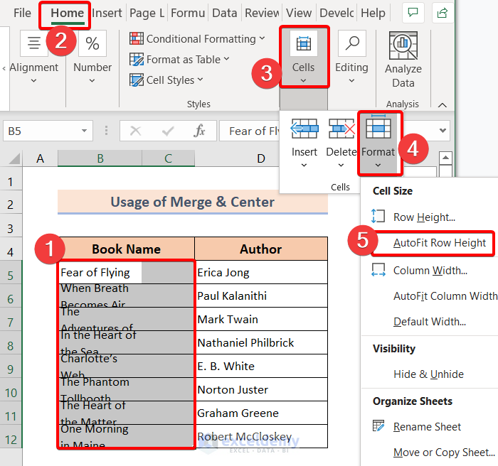
Method 1 - Apply AutoFit Row Height Command to Fix Wrap Text Not Showing All Text We applied the Wrap Text command in the Book Name column. The texts are not ...
Method 1 - Using the LEN Function and a Helper Column Steps: Create a Helper column left to the main data table. Enter the following formula in the ...

Excel offers changing cases in Excel either using a formula or without even using formulas. In this article, you will learn 5 ways to change cases in Excel ...

Method 1 - Using Find and Replace to Remove Text from Excel Cell but Leave Numbers Steps: Create a helper column. Copy the values from the ...

Microsoft Excel offers multiple ways to add dashes to social security numbers (SSNs), including using formulas or the Format Cells dialog box. In this article, ...

Method 1 - Combine the VLOOKUP and CHOOSE Functions to Vlookup with Multiple Criteria in Excel ❶ Select cell G9 first. ❷ Then insert the following formula: ...

Basically, formulas are an essential component of Excel, as they allow users to perform complex calculations and automate tasks. But, while sharing your ...

Step 1 - Set up a Unique List to Create a Drop-Down List Filter Based on the Cell Value in Excel Copy the data. Here, the data in the Category column. ...
- « Previous Page
- 1
- …
- 4
- 5
- 6
- 7
- 8
- …
- 12
- Next Page »
See Our Reviews at


Thanks for your feedback.
Hello Mr. Mejon,
Unfortunately, there is no VBA function that calculates the probability of area left to a Z score in a skewed distribution.
However, I’m suggesting you some functions that might help you.
Z.TEST function >>> Returns the one-tailed probability-value of a z-test.
KURT function >>> Returns the kurtosis of a data set.
GAUSS function >>> Returns 0.5 less than the standard normal cumulative distribution.
F.DIST.RT function >>> Returns the F probability distribution.
SKEW.P function >>> Returns the skewness of a distribution based on a population: characterization of the degree of asymmetry of a distribution around its mean.
Regards!
Hi Shabbir,
Thanks for your nice words!
Best regards.
Hi Brenda,
Follow this tutorial to fetch all the data tables from a web page. After selecting a particular data table, click on the Transform Data command to modify your data table in the Power Query Editor. There you can remove all the unnecessary columns and keep your desired data. Then hit the Close & Load button to bring the transformed data table into your worksheet.
Thanks.
Hi Anthon,
If there’s no data table on a web page, Excel will import a default document data table into the worksheet. The document table is basically a null data table.
Hi Ron,
You can see that yellow square with a red arrow in Microsoft Office Professional Plus 2016. In Excel 2019, you won’t find that because there’s no need to use the yellow box. Excel will automatically detect all the tables and make a list of ’em. All you need to do is, simply select any of the tables that you want to import and then load them directly into your Excel worksheet.
Thanks!
Hi Jennifer,
I think you have issues with your dates. Make sure your dates are accurate and in proper date format. Confirming your dates, you can apply the WEEKDAY function again. Still, if you suffer from this problem, it’s better to check the format that you’ve applied. To highlight Sunday you will apply the following formula: =WEEKDAY(B4:B12)=1. Make sure that the range inside the WEEKDAY function is legit. If everything goes just fine, this formula will highlight all the Sundays throughout your dates.
If nothing works for you, I would suggest you send your Excel file to my mail address: [email protected]. I will see what’s wrong with your data.
Thanks!
Hi KEITH,
Your problem is partly vague I think. Still, I’ve tried to build a formula that might work for you. If this doesn’t work, I would recommend you share your workbook with me or at least share a sneak peek of your dataset.
Now use this formula:
=IF(ISBLANK(K2),SUMIF(I2:I13,”asphalt field”,N2:N13),SUM(J2:J13,L2:L13))
Thanks!
Hi GVS,
This is Mrinmoy. I’m replying to you on behalf of Mr. Rifat. Currently, he has been shifted to another project. If you don’t mind, you can send your file to my email address at [email protected]. I will try to help you as much as possible.
Regards!
Hi Michelle,
You can try the following piece of code:
Sub PasteAcrossSheets()
Dim arr(3)
i = 0
For Each Worksheet In ActiveWorkbook.Sheets
Worksheet.Activate
arr(i) = ActiveSheet.Name
i = i + 1
Next
yy = ActiveWindow.RangeSelection.Address
Set xx = Application.InputBox(“Insert a range:”, “Microsoft Excel”, yy, , , , , 8)
If xx Is Nothing Then Exit Sub
mm = Application.ScreenUpdating
Application.ScreenUpdating = False
xx.Copy
Sheets(arr).Select
Range(“G5”).Select
ActiveSheet.Paste
Application.CutCopyMode = False
Application.ScreenUpdating = mm
End Sub
Hi Scot,
The following code may fulfill your requirements.
Sub TextHighlighter()
Application.ScreenUpdating = False
Dim Rng As Range
Dim cFnd As String
Dim xTmp As String
Dim x As Long
Dim m As Long
Dim y, ext As Long
cFnd = InputBox(“Enter the text string to highlight”)
Color_Code = Int(InputBox(“Enter the Color Code: ” + vbNewLine + “Enter 3 for Color Red.” + vbNewLine + “Enter 5 for Color Blue.” + vbNewLine + “Enter 6 for Color Yellow.” + vbNewLine + “Enter 10 for Color Green.”))
ext = CLng(InputBox(“Input number of additional Character to color”, , 0))
y = Len(cFnd) + ext
For Each Rng In Selection
With Rng
m = UBound(Split(Rng.Value, cFnd))
If m > 0 Then
xTmp = “”
For x = 0 To m – 1
xTmp = xTmp & Split(Rng.Value, cFnd)(x)
.Characters(Start:=Len(xTmp) + 1, Length:=y).Font.ColorIndex = Color_Code
xTmp = xTmp & cFnd
Next
End If
End With
Next Rng
Application.ScreenUpdating = True
End Sub
Hi CHRIS,
Thanks for this interesting question. It’s not about adding multiple COUNTIFS functions but multiple COUNTIF functions inside one IFS function.
Look at the following formula. It will look for two keywords “MTT” and “GL” across the text. If it finds MTT then the output will be “MTT Exists!”. For “GL” the output will be “GL Exists!”.
If nothing matches, it will return “No Results Found!”.
=IFERROR(IFS(COUNTIF(B5,”*MTT*”),”MTT Exists!”,COUNTIF(B5,”*GL*”),”GL Exists!”),”No Results Found!”)
Regards!
Hi Les,
Conditional Formatting is a static feature. Being a static feature, it doesn’t update itself automatically. However, you can apply the conditional formatting again with the default cell color to unhighlight all the completed dates.
Regards!
Hi Andrew,
It happens because of the variable types. The two variables X & Y currently have the variable type “Long” and “Integer” respectively. To get a sum value up to 2 decimal places, make both variable types “Double”. This will reserve the decimal places.
Here’s the modified code:
Function SumColoredCells(CC As Range, RR As Range)
Dim X As Double
Dim Y As Double
Y = CC.Interior.ColorIndex
For Each i In RR
If i.Interior.ColorIndex = Y Then
X = WorksheetFunction.Sum(i, X)
End If
Next i
SumColoredCells = X
End Function
I hope this will work. Regards!
Hi Joris,
The Me keyword can’t appear in a standard module because a standard module doesn’t represent an object. If you copied the code in question from a class module, you have to replace the Me keyword with the specific object or form name to preserve the original reference.
Thanks!
Hi SAM,
The first formula: =LOOKUP(2,1/($B$5:$B$12=$B$15),$C$5:$C$12) returns #N/A error for a lookup value that cannot be found. Thus, you can add the IFERROR function to tackle this issue.
For example use the following formula to return “Null” instead of #N/A error: =IFERROR(LOOKUP(2,1/($B$5:$B$12=$B$15),$C$5:$C$12),”Null”)
I hope this is what you were looking for.
Regards!
Hello Katherine,
This is a critical issue. The 4 solutions provided above are all the known solutions you will find on the internet.
So make sure, you’ve tried all the solutions accurately. Yet, you can emphasize more on solution no 2. As you described, you are facing this problem suddenly. Chances are your worksheet contains a graphic object that is invisible. So, try to find it out and remove it.
Still, if it doesn’t work properly, then you can start over with a new workbook.
Regards!
Hi Larry Kanzia,
Inverted commas can be single – ‘x’ – or double – “x”. They are also known as quotation marks, speech marks, or quotes.
You can get a single inverted comma just by pressing the comma button next to the ENTER button on your keyboard. To insert a double inverted comma, press and hold the SHIFT key, then press the comma key next to the ENTER button.
Thanks!
Hello Nicholas,
There’s no easy way to make a User-Defined Function dynamic. However, you can use an event procedure using the Worksheet_SelectionChange event to recalculate each time you change cell color. This will recalculate the formula whenever you prompt an event in your worksheet.
But I don’t recommend you to use this technique. Because it’ll slow down your workflow in Excel. Using the event procedure, the UDF will continue to calculate each time you click on your sheet.
However, you can press CTRL + ALT + F9 to recalculate manually each time you change cell color. It’s the best solution to your problem so far.
Regards!
Hello Mr. Masud,
You can easily solve your problem by combining the IF and AND functions.
Suppose, you have 3 values to compare in three cells C7, D7, and E7. For this instance, let’s say C7 is in sheet1, D7 is in sheet2, and E7 is in sheet3.
Now you are in sheet3 and you want to get a feedback (Yes or No) in cell F7.
All you need to do is, type the following formula in cell F7 of sheet3.
=IF(AND(Sheet1!C7=Sheet2!D7,Sheet2!D7=Sheet3!E7),”Yes”,”No”)
After that, press ENTER and you will get your required result.
Regards!
Hello Mr. Fazal,
You can download the attached Excel file and use that as a template.
All you need to do is input the number of years, periods per year, and balance. All the columns have their corresponding formula applied. As you provide the required information, Excel will automatically calculate the Loan Amortization Schedule for you.
Last but not the least, you have to update the variable annual interest rate (AIR) manually. If you have any lump sum amount in your consideration don’t forget to update that too!
Regards!