Latest Posts From Eshrak Kader

Consider the dataset containing a List of Decimal Numbers. To convert these decimal numbers into binary numbers: Method 1 - Using the ...
What Is a Data Model? In simple terms, a Data Model enables us to combine information from many tables to create a relational data source within an Excel ...

Consider the Sales Dataset containing Items and Sales in USD. Step 1 - Insert a Treemap chart Go to the Insert tab >> click Insert ...
Indeed, Excel has a powerful graphing feature that can add visual depth and clarity to even the most boring of datasets. For instance, you may want to make a ...

Indeed, Microsoft Excel is renowned for managing and manipulating data; However, formatting text is also an essential aspect of data analysis. What if you need ...
The dataset showcases the Population Growth in The USA. Using the above dataset, you’ll get the following graph. To add data points to ...
![[Fixed!] Cursor Selecting Wrong Cell in Excel (6 Proven Solutions)](https://www.exceldemy.com/wp-content/uploads/2022/11/How-to-Fix-Cursor-Selecting-Wrong-Cell-in-Excel-2.1-1.png?v=1697441937)
Here are the Quarterly Sales Data for 2021 shown in the B4:F14 cells, containing the Location and the four Quarters Q1, Q2, Q3, and Q4, respectively. We want ...
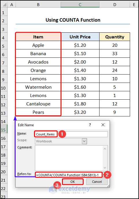
The sample dataset (B4:D13) showcases Item, Quantity, and Unit Price of Fruit Sales. Example 1: Multiplying Named Ranges Steps: Go ...

Method 1 - Nesting Two COUNTIF Functions Steps: Go to the D16 cell >> enter the formula given below. ...

Dataset Overview Consider the List of Employees and Departments dataset shown in cells B4:D14. This dataset includes employee IDs, their Names, and the ...
![[Fixed!] Excel Scroll Bar Too Long: 5 Methods](https://www.exceldemy.com/wp-content/uploads/2022/10/Excel-Scroll-Bar-Too-Long-4.3-1.png?v=1697435820)
Method 1 - Deleting Contents from Other Cells Steps: Consider we have some unwanted text in the B1048563 cell. Click on column F to select the ...

Unquestionably, Microsoft Excel and Google Sheets are two of the most useful and popular tools for data analysis. Though you can easily download Google Sheets ...
To illustrate, let's assume the Fruit Sales Data shown in the B4:E13 is what we want to copy and paste from Excel to Google Sheets. Method 1 - Using ...

This article shows a step-by-step guide on how to edit VCF file in Excel, as well as in Notepad. We have used the Microsoft 365 version of Excel here, but ...

Undoubtedly, Excel is a popular and useful tool for summarizing large sets of data. Now, wouldn’t it be great if we could attach documents in Excel? Sounds ...
- « Previous Page
- 1
- 2
- 3
- 4
- 5
- …
- 8
- Next Page »
See Our Reviews at


Hello Philip Earland,
Thank you for your query. You can find the answer to your question in the Excel file linked to this message. The steps are described below.
Bank Reconciliation.xlsx
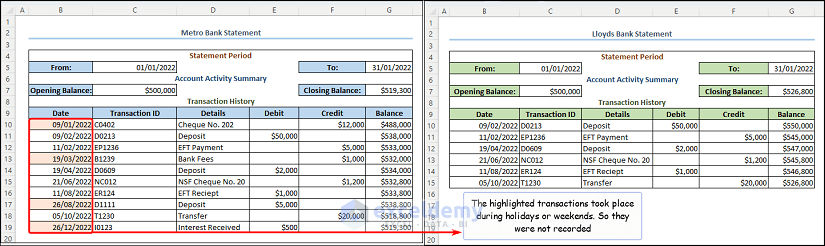
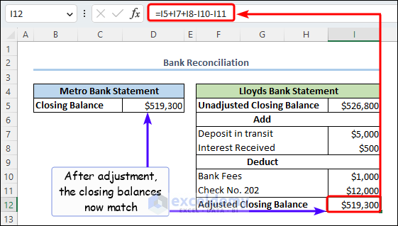
Consider the transactions from “Metro Bank” to “Lloyds Bank”. We can see the closing balances are not the same and need to be reconciled.
Select the transaction dates in the B10:B19 cells >> click the Conditional Formatting drop-down >> go to New Rule.
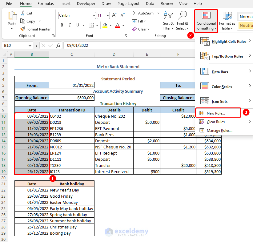
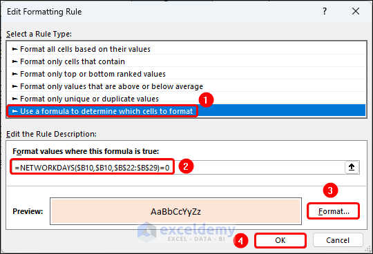
Select Use a formula to determine which cells to format option >> enter the formula given below >> select fill color, here we’ve chosen the color “Orange, Accent 2, Lighter 80%”.
=NETWORKDAYS($B10,$B10,$B$22:$B$29)=0Here, the highlighted transactions were processed by “Metro Bank” just before the weekends or holidays, so they were not recorded in the “Lloyd Bank” statement.
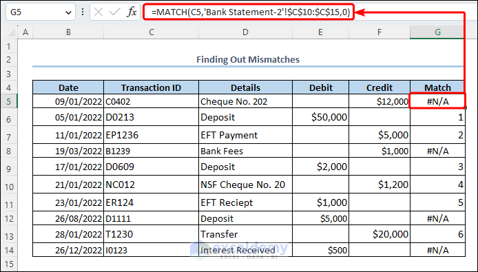
Next, move to the “Mismatch” worksheet and apply the MATCH function to find the discrepancies between the two statements. Here the #N/A errors are the mismatches.
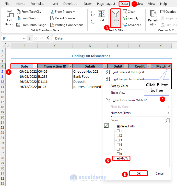
Then, use the Filter option in the Data tab to show only the mismatches.
Enter the mismatched account names and their amounts >> apply the expression below to reconcile the differences.
=I5+I7+I8-I10-I11Hope this helps. Have a good day.
Regards,
Exceldemy
Hello Jeff,
Thank you for your query. You can find the answer to your question in the Excel file linked to this message.
Sort Alphanumeric.xlsx
Follow the steps shown below to sort alphanumeric data.
Enter the formula into the E5 cell to convert the alphanumeric data to numeric data >> drag the Fill Handle tool to copy the formula to the cells below.
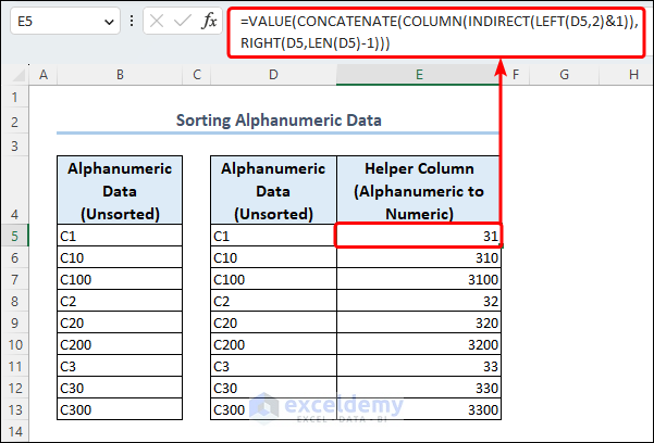
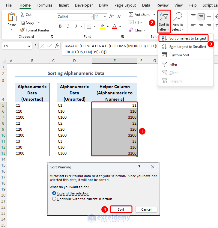
=VALUE(CONCATENATE(COLUMN(INDIRECT(LEFT(D6,2)&1)),RIGHT(D6,LEN(D6)-1)))Now, select the E5:E13 range >> click Sort & Filter >> select Sort Smallest to Largest.
A warning box appears, Expand the selection option is checked by default >> click the Sort button.
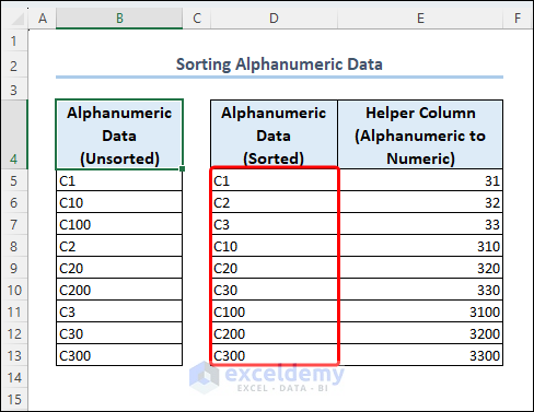
That’s it the data will be sorted.
Hope you find this useful. Have a good day.
Regards,
ExcelDemy.
Hello Nimesh,
Thank you for your query. You can find the answer to your question in the Excel file linked to this reply.
Counting Significant Figures.xlsx
Here is a screenshot of the results in the Excel file.
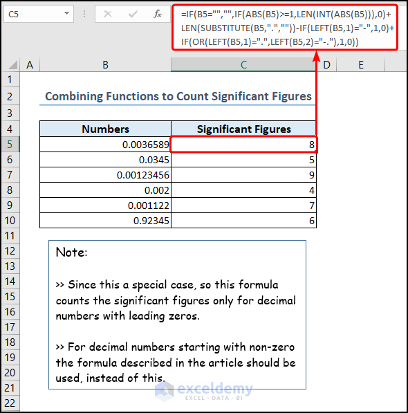
Hope you this useful. Have a good day.
Regards,
ExcelDemy
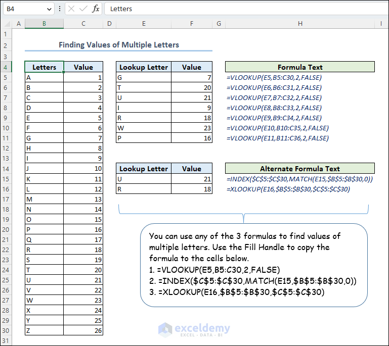
Hello Saccharine,
Thank you for your query. You can find the answer to your question in the Excel file attached to this message.
How to Find Values of Multiple Letters.xlsx
Here is a sample image of the Excel file.
Hope this helps. Have a good day.
Regards,
Exceldemy
Hello Avinash,
Thank you for your query. We have attached an Excel file with the answer to your question. Make sure to download the file.
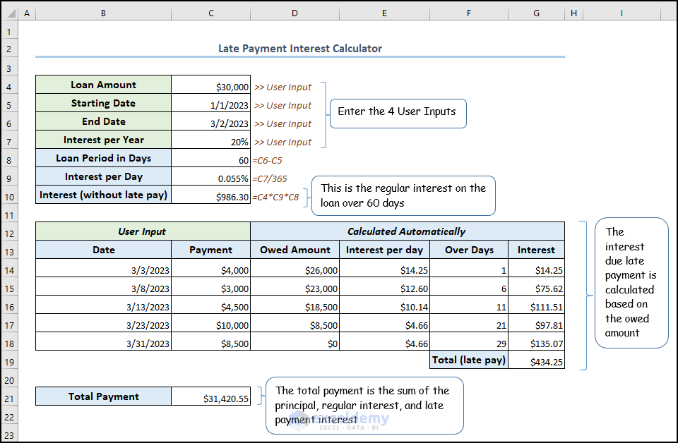
Late Payment Interest Calculator.xlsx
Here is a snapshot from the Excel file.
Hope this helps. Have a good day.
Regards,
ExcelDemy
Hello Tomás Limeme,
Thank you for your feedback. The goal of a bank reconciliation is to identify and adjust any difference between the closing balances of our cashbook and bank statement over a specific period. To do this, we add or subtract any unrecorded transaction from our unadjusted closing balance.
In short, adding and subtracting ensures the matching of the bank statement and cashbook balances. This is important for proper financial reporting and to avoid mistakes or fraud.
Let’s review some of the transactions that are added, followed by the transactions that are subtracted.
Examples of transactions that are added include:
1. Deposits in transit: Funds transferred to the bank account but not yet entered into the accounting system.
2. Bank errors: Mistakes made by the bank, such as incorrectly recorded deposits or credits.
3. Earned interest: Interest on an account that hasn’t been entered into the accounting system.
On the other hand, subtracted transactions are:
1. Outstanding checks: Checks that have been written but have not yet been cashed by the bank.
2. Bank fees: Charges made by banks that are not accounted for in the accounting system.
3. Not Sufficient Fund checks: Checks that the bank returned due to insufficient money in the account of the issuer.
Hope this helps, have a good day.
Regards,
ExcelDemy
Hello AFIF,
Thank you for your question. Yes, we can perform the vehicle life cycle cost analysis for a duration of 25 years; just change the period of ownership to 25 and Excel should automatically show the updated results.
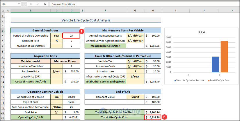
We have also included the Excel file with this message for you to download.
Vehicle-Life-Cycle-Cost-Analysis.xlsx
Regards,
ExcelDemy
Thank you for your inquiry. Regrettably, Microsoft Word does not have the capability to perform a mail merge with Excel charts. Although there are third-party add-ins that claim to provide this functionality, we cannot vouch for their security, and therefore, we do not recommend their use.
Perhaps, you may post this query on Microsoft Community, where experts can direct you to a trusted alternative.
Regards,
ExcelDemy
Hello Bruce,
Thank you for your feedback and for pointing out the error. In this case, instead of Coupons it should be Coupon Payment which in this case has been considered $30.0 as shown in the updated picture below.
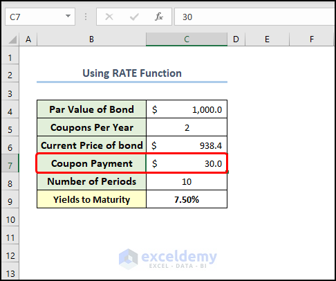
Hopefully, this clears out any confusion and we are sorry for this error.
Regards,
ExcelDemy
Hello KC,
Thanks for the feedback. It appears that the INDIRECT function is unable to return the sum of two columns from multiple worksheets, even though it works fine for a single column. Rather, we can use the XLOOKUP and SUM functions to get the results.
You can download the Excel file included in this reply.
SUMIF Across Multiple Sheets.xlsx
Consider the Sales Performance dataset for Los Angeles, likewise, we have the Sales Performance dataset for New York.
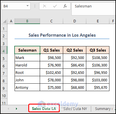
The screenshot below shows the aggregate sales for each salesman using the SUM and XLOOKUP functions.
=SUM(XLOOKUP(B5,'Sales Data LA'!$B$4:$B$9,'Sales Data LA'!$C$4:$E$9),
XLOOKUP(B5,'Sales Data NY'!$B$4:$B$9,'Sales Data NY'!$C$4:$E$9))
Regards,
ExcelDemy
Hello CHRISP,
Thank you for your question, we have included a screenshot of the results and you can find the Excel file linked below.
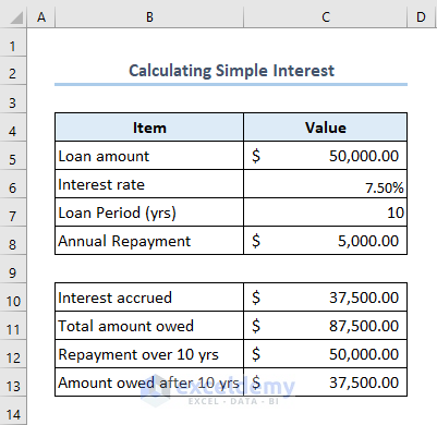
Calculating Simple interest.xlsx
Regards,
ExcelDemy
Hello RICHARD MUTALE BWALYA,
Thank you for your question. Changing a fixed-rate loan to a variable rate depends on the terms and conditions of the loan agreement, in addition to the applicable laws and regulations in the jurisdiction where the loan was made.
So, we believe it is best that you contact a financial advisor who can suggest the proper course of action based on your agreement.
Regards,
ExcelDemy
Hello KLC,

Thank you for your feedback. Unfortunately, we’re having trouble accessing the pictures in the link, so you can attach your Excel workbook and send it to us at [email protected].
Regards,
ExcelDemy
Hello SAM,
We have attached an Excel file with this reply which you can download from the link below.
Print-Sheets-Using-Excel-Button.xlsm
Here, we’ve modified the code such that it automatically lists the names of the worksheets when opened. You can select multiple worksheets and press the print button to print them.
Regards,
ExcelDemy
Hello JOE,
Thank you for your feedback. Did you try the solutions suggested in the article and did they work before 6 February 2023?
If the solutions worked before, then you may need to repair your Microsoft Office application.
Hopefully, this resolves the problem.
Regards,
ExcelDemy
Hello ROSEMARIE LINFOOT,
We have attached an Excel workbook with the necessary instructions to this reply. You can download the file using the link below.
Loan-Amortization-Schedule-with-Variable-Interest-Rate-And-OCR.xlsx
If you have further queries please attach a sample workbook and contact us at [email protected].
Regards,
ExcelDemy
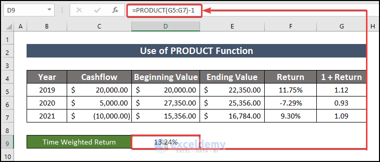
Hello DAN,
Firstly, we would like to apologize for the trouble. As you pointed out, the use of the GEOMEAN function does not return the correct answer. In fact, we can apply the PRODUCT function as shown below.
=PRODUCT(G5:G7)-1Here, the G5:G7 range refers to the values in the “1+Return” column.
Regards,
ExcelDemy
Hello SHABBIR,
You can follow a step-by-step guide or use the free template for your simple accounting system by following this article on How to do Bookkeeping for Small Businesses.
Regards,
ExcelDemy
Hello DONNA ATKINS,
Thank you for your feedback, the answer to your question is provided in the steps below, so follow along.
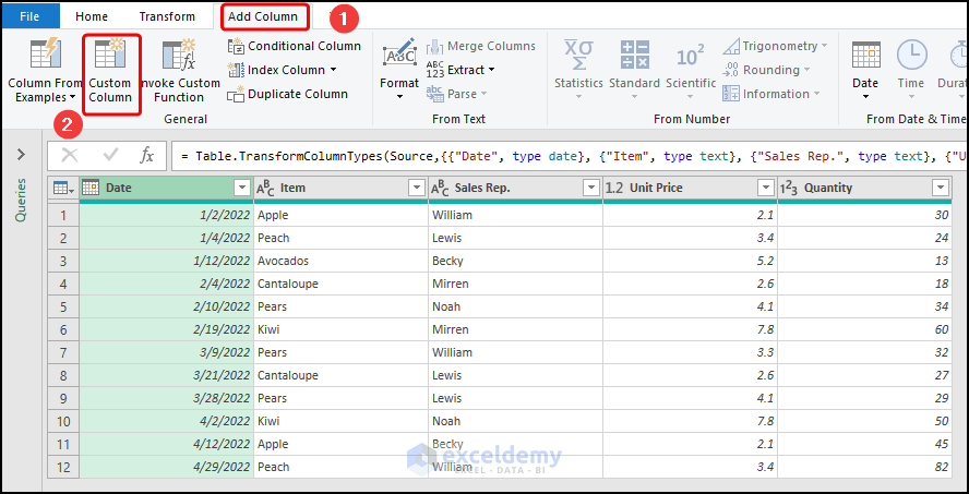
Step 1. First, complete steps 1 through 5 from Method 1 >> now, follow the steps shown in the live demonstration.
Step 2. Next, click on Close & Load drop-down >> select Close & Load to option.
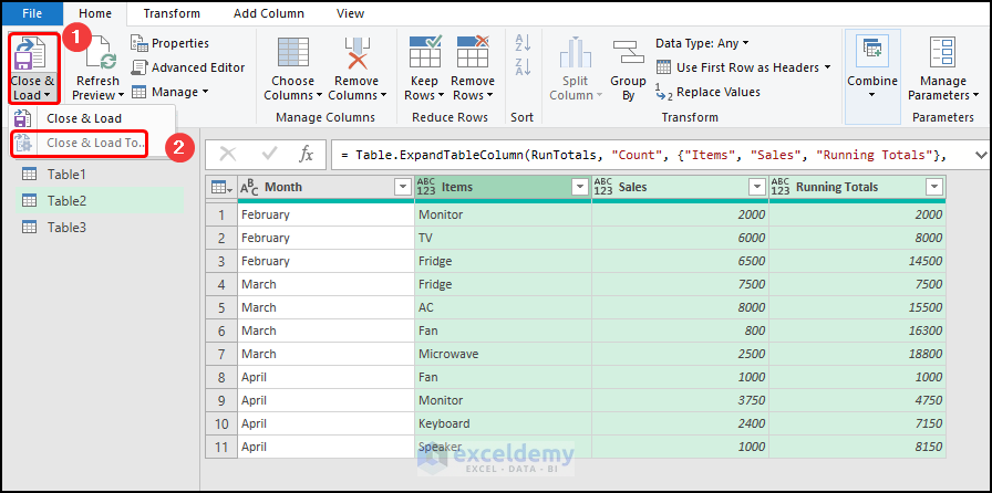
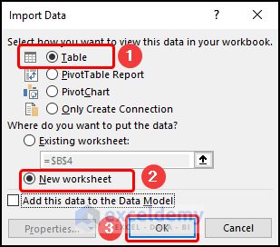
Step 3. Lastly, choose the Table or PivotTable option according to your preference >> load this data into a new worksheet.
Hopefully, this solves your problem. Have a good day.
Hello KAREN W,
First of all, we would like to apologize for the trouble. As you pointed out, there were in fact some issues with the cell referencing in the Regression mathod, luckily they have been updated.
The Exceldemy team is grateful to you for sharing your thoughts and feedback. Hopefully, now you can obtain the desired result.
Hello JB,
Thank you for your feedback. Admittedly, like everything else, Excel has its downsides too and sometimes the solution to a problem can be quite surprising, but whatever works! Right?
That said, we’re delighted that you’ve shared your experience with us, hopefully, other people find this useful. Have a good day.
Hello Behzad,
Thank you for your question. We’re sorry to hear that you’re facing difficulties with the formula. In fact, the ExcelDemy team has tested the Excel file following your comment and the formula appears to be working correctly.
That said, it would be helpful if you could send us a screenshot of the issue that you’re experiencing.
Hello S,
Thank you for your question. Firstly, I would like to apologize for the misunderstanding. Admittedly, the method in question is in fact a quick and dirty way to manually insert page numbers if your document contains only a handful of pages.
That said, the widely accepted process of inserting page numbers in Excel is described in Method 4. Hopefully, this helps.
Hello Jamil Khan,
Thank you for your question. Actually, this is how the RANK function works, that is to say, it ranks the duplicate values in ascending or descending order according to the given argument. Now, to have the same ranks for identical values you can follow Method 1 or download the Excel file that the ExcelDemy team has created.
Download the Excel File below.
Ranking Duplicates.xlsx
Hello Phong,
Thank you for your suggestion and for taking the trouble to provide a great solution to Kate’s problem. We, the ExcelDemy team really appreciate your effort and as a result, we’ve updated our article to include the solution that you’ve provided.
Hello P.KUIPERS,
Thank you for your question. The ExcelDemy team has created an Excel file with the solution to your question that you may download from the link below.
Rename_Sheets.xlsm
You can download the practice files from the link below
Rename_Sheets_Do_Yourself.xlsm
Otherwise, you can just follow the steps below.
In order to rename the sheets in a sequential way, you can use another VBA Macro. So, let’s see the step below.
Step: 1
a. Firstly, navigate to the Developer tab >> click the Visual Basic button. This opens the Visual Basic Editor in a new window.
b. Next, go to the Insert tab >> select Module.
For your ease of reference, you can copy the code from here and paste it into the window.
Sub Rename_Multiple_Sheets()
Alphabets = Array(“A”, “B”, “C”, “D”, “E”, “F”, “G”, “H”, “I”, “J”, “K”, “L”, “M”, “N”, “O”, “P”, “Q”, “R”, “S”, “T”, “U”, “V”, “W”, “X”, “Y”, “Z”)
Days = Array(“Monday”, “Tuesday”, “Wednesday”, “Thursday”, “Friday”, “Saturday”, “Sunday”)
Dim Weekdays(5) As String
For i = 0 To 4
Weekdays(i) = Days(i)
Next i
Months = Array(“January”, “February”, “March”, “April”, “May”, “June”, “July”, “August”, “September”, “October”, “November”, “December”)
Old_Names = InputBox(“Enter the Names of the Worksheets to Change (Separate them be Commas).” + vbNewLine + “OR” + vbNewLine + “Enter ALL to change all the worksheets.”)
If Old_Names = “ALL” Then
Dim Old_Sheets() As String
ReDim Old_Sheets(Sheets.Count – 1)
For i = 0 To Sheets.Count – 1
Old_Sheets(i) = Sheets(i + 1).Name
Next i
Else
Old_Sheets = Split(Old_Names, “,”)
End If
Dim Used_Names() As String
ReDim Used_Names(0)
Dim Sign As Integer
Sequential_Or_Random = Int(InputBox(“Enter 1 to Change the Worksheet Names in a Sequential Way: ” + vbNewLine + “OR” + vbNewLine + “Enter 2 to Change the Worksheet Names in a Random Way: “))
If Sequential_Or_Random = 1 Then
Series = Int(InputBox(“Enter 1 to Change the Names to a Series of Numbers: ” + vbNewLine + “Enter 2 to Change the Names to a Series of ALphabets: ” + vbNewLine + “Enter 3 to Change the Names to a Series of Days: ” + vbNewLine + “Enter 4 to Change the Names to a Series of Weekdays: ” + vbNewLine + “Enter 5 to Change the Names to a Series of Months: “))
If Series = 1 Then
Prefix = InputBox(“Enter the Prefix before the Numbers: “)
First_Number = Int(InputBox(“Enter the First Number: “))
Increment = Int(InputBox(“Enter the Increment: “))
For i = 0 To UBound(Old_Sheets)
Sheets(Old_Sheets(i)).Name = Prefix + Str(First_Number + Increment * (i))
Next i
ElseIf Series = 2 Then
Prefix = InputBox(“Enter the Prefix before the Letters: “)
First_Letter = InputBox(“Enter the First Letter: : “)
Increment = Int(InputBox(“Enter the Increment: “))
Dim Case_Identifier As String
For i = 0 To UBound(Alphabets)
If Alphabets(i) = First_Letter Then
First_Letter_Number = i
Case_Identifier = “U”
Exit For
ElseIf LCase(Alphabets(i)) = First_Letter Then
First_Letter_Number = i
Case_Identifier = “L”
Exit For
End If
Next i
For i = 0 To UBound(Old_Sheets)
Sign = 0
For j = 0 To UBound(Used_Names)
If Alphabets((First_Letter_Number + (Increment * i)) Mod 26) = Used_Names(j) Then
Sign = Sign + 1
End If
Next j
If Sign = 0 Then
If Case_Identifier = “U” Then
Sheets(Old_Sheets(i)).Name = Prefix + Alphabets((First_Letter_Number + (Increment * i)) Mod 26)
Else
Sheets(Old_Sheets(i)).Name = Prefix + LCase(Alphabets((First_Letter_Number + (Increment * i)) Mod 26))
End If
Else
If Case_Identifier = “U” Then
Sheets(Old_Sheets(i)).Name = Prefix + Alphabets((First_Letter_Number + (Increment * i)) Mod 26) + ” (” + Str(Sign) + “)”
Else
Sheets(Old_Sheets(i)).Name = Prefix + LCase(Alphabets((First_Letter_Number + (Increment * i)) Mod 26)) + ” (” + Str(Sign) + “)”
End If
End If
ReDim Preserve Used_Names(i)
Used_Names(i) = Alphabets((First_Letter_Number + (Increment * i)) Mod 26)
Next i
ElseIf Series = 3 Then
First_Day = LCase(InputBox(“Enter the First Day: : “))
Increment = Int(InputBox(“Enter the Increment: “))
For i = 0 To UBound(Days)
If LCase(Days(i)) = First_Day Then
First_Day_Number = i
Exit For
End If
Next i
For i = 0 To UBound(Old_Sheets)
Sign = 0
For j = 0 To UBound(Used_Names)
If Days((First_Day_Number + (Increment * i)) Mod 7) = Used_Names(j) Then
Sign = Sign + 1
End If
Next j
If Sign = 0 Then
Sheets(Old_Sheets(i)).Name = Days((First_Day_Number + (Increment * i)) Mod 7)
Else
Sheets(Old_Sheets(i)).Name = Days((First_Day_Number + (Increment * i)) Mod 7) + ” (” + Str(Sign) + “)”
End If
ReDim Preserve Used_Names(i)
Used_Names(i) = Days((First_Day_Number + (Increment * i)) Mod 7)
Next i
ElseIf Series = 4 Then
First_Weekday = LCase(InputBox(“Enter the First Day: : “))
Increment = Int(InputBox(“Enter the Increment: “))
For i = 0 To UBound(Weekdays)
If LCase(Weekdays(i)) = First_Weekday Then
First_Weekday_Number = i
Exit For
End If
Next i
For i = 0 To UBound(Old_Sheets)
Sign = 0
For j = 0 To UBound(Used_Names)
If Weekdays((First_Weekday_Number + (Increment * i)) Mod 5) = Used_Names(j) Then
Sign = Sign + 1
End If
Next j
If Sign = 0 Then
Sheets(Old_Sheets(i)).Name = Weekdays((First_Weekday_Number + (Increment * i)) Mod 5)
Else
Sheets(Old_Sheets(i)).Name = Weekdays((First_Weekday_Number + (Increment * i)) Mod 5) + ” (” + Str(Sign) + “)”
End If
ReDim Preserve Used_Names(i)
Used_Names(i) = Weekdays((First_Weekday_Number + (Increment * i)) Mod 5)
Next i
ElseIf Series = 5 Then
First_Month = LCase(InputBox(“Enter the First Month: “))
Increment = Int(InputBox(“Enter the Increment: “))
For i = 0 To UBound(Months)
If LCase(Months(i)) = First_Month Then
First_Month_Number = i
Exit For
End If
Next i
For i = 0 To UBound(Old_Sheets)
Sign = 0
For j = 0 To UBound(Used_Names)
If Months((First_Month_Number + (Increment * i)) Mod 12) = Used_Names(j) Then
Sign = Sign + 1
End If
Next j
If Sign = 0 Then
Sheets(Old_Sheets(i)).Name = Months((First_Month_Number + (Increment * i)) Mod 12)
Else
Sheets(Old_Sheets(i)).Name = Months((First_Month_Number + (Increment * i)) Mod 12) + ” (” + Str(Sign) + “)”
End If
ReDim Preserve Used_Names(i)
Used_Names(i) = Months((First_Month_Number + (Increment * i)) Mod 12)
Next i
End If
ElseIf Sequential_Or_Random = 2 Then
New_Names = InputBox(“Enter the New Names (Separate them by Commas): “)
New_Sheets = Split(New_Names, “,”)
For i = 0 To UBound(Old_Sheets)
Sign = 0
For j = 0 To UBound(Used_Names)
If New_Sheets(i) = Used_Names(j) Then
Sign = Sign + 1
End If
Next j
If Sign = 0 Then
Sheets(Old_Sheets(i)).Name = New_Sheets(i)
Used_Names(Count) = New_Sheets(i)
Count = Count + 1
Else
Sheets(Old_Sheets(i)).Name = New_Sheets(i) + ” (” + Str(Sign) + “)”
End If
ReDim Preserve Used_Names(i + 1)
Used_Names(i + 1) = New_Sheets(i)
Next i
End If
End Sub
Step: 2
a. Secondly, close the Visual Basic Editor >> in the top Ribbon, click the Macros button >> Now, select the Rename_Multiple_Sheets Macro and press Run.
b. This opens up a few input boxes. The inputs are described in the step below therefore just follow these steps.
Step: 3
a. The first Input Box will ask you to enter the name of the sheets that you want to change. Since you want to rename your worksheets to Sheet1, Sheet2, etc. you can type in ALL.
b. The second Input Box will ask you whether you change the sheet names in a sequential way or in a random way. In this case, you enter 1.
c. If you go for a sequential way, the third Input Box will ask for a series of values from the options below. Now, enter 1 for a series of Numbers (1, 2, 3, etc.)
d. Next, enter a Prefix before the numbers, for instance, “Sheet”.
e. Then, give the Starting Number, in this case, 1.
f. Lastly, provide the Increment for the numbers, for example, you can choose 1.
Voila! All your sheets are numbered serially as Sheet 1, Sheet 2, etc.
If you wish you can learn more about this VBA Code in this article.
Hello Julie Parker,
Thank you for your question. I have looked into this matter, and so far, I haven’t been able to find a solution to your particular query. In the meantime, I have prepared an excel template with a table of contents that you may download from the link below. That said, I will let you know when I find a solution. I hope this was helpful.
Table of Contents.xlsx
Hello RAY,
Thank you for your question. The Exceldemy team has created an Excel file with the solution to your question. Please provide your email address here, we will send it to you in no time.
Otherwise, you can just follow the steps below.
Suppose we want to use the MID Function as shown in Method 1. Now, we want to determine the age of a person whose ID Number starts with 00 (which refers to the Year 2000) but that person was born after the Year 2000.
Step: 1
• Firstly, let’s consider Mary with the ID Number to be ‘0005255800012.
• As a note, Excel removes any leading zeros from numbers so we have inserted an apostrophe comma to store the ID Number as text.
Step: 2
• Secondly, let’s assume Mary was born in the Year 2003.
• Now, on the Date of Birth column insert the formula given below.
=MID(C14,5,2)&"/"&MID(C14,3,2)&"/"&"0"&MID(C14,1,2)+3• You should see the result as 25/05/03.
Step: 3
• Next, AutoFill the Current Date and Age columns.
• The value of Age should be 19 years.
Similarly, we have also included a second example for Julian with the ID Number ‘0108295800012 but he was born in the Year 2006.
Please feel free to provide any further feedback.
Hello KATE,
Thank you for your question. You can reduce a fraction to its lowest term by specifying the format style of the TEXT function to: =INT(C5) & ” ft ” &TEXT(MOD(C5,1)*12, “000/00”.) & “in”
Hello FELICIA FOO,
Thank you for your question. You can find the average of a group by right-clicking on the Row Labels (Sum of Sales) and selecting the Value Field Settings option. Next, in the Summarize value field by list, you’ll find Average.