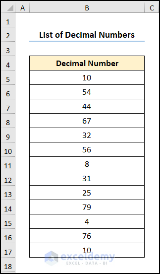
Consider the dataset containing a List of Decimal Numbers.
To convert these decimal numbers into binary numbers:
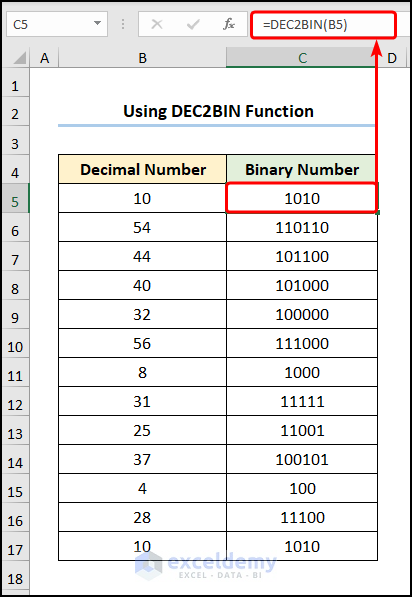
Method 1 – Using the DEC2BIN Function
Steps:
- Go to C5 >> enter the formula >> use the Fill Handle Tool to copy the formula into the cells below.
=DEC2BIN(B5)
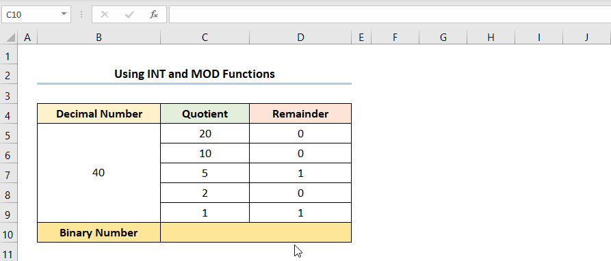
B5 refers to the value of a “Decimal Number” : 10.
This is the output.
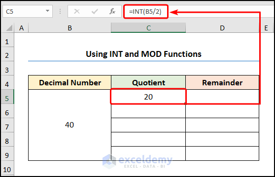
Method 2 – Utilizing the INT and MOD Functions
Steps:
=INT(B5/2)
B5 indicates the “Decimal Number”: 40.
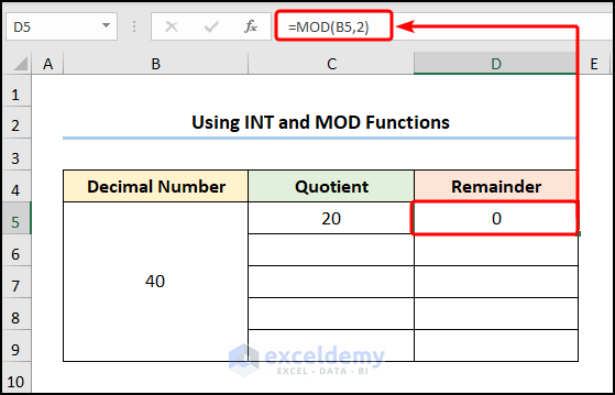
- Go to the adjacent D5 >> use the equation below.
=MOD(B5,2)
B5 represents the “Decimal Number” :“40” and 2 is the divisor.
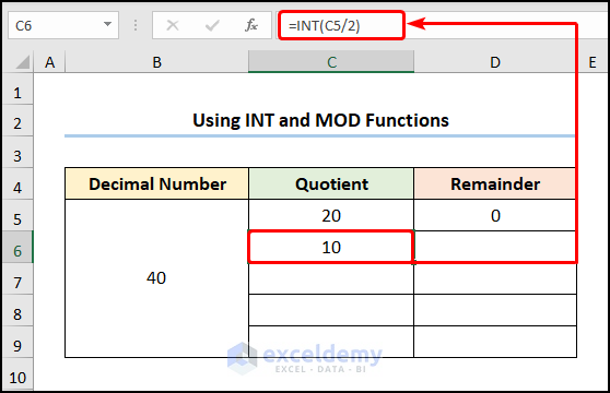
- Enter the following equation in C6.
=INT(C5/2)
C5 is the “Quotient”: 20.
- Copy the formula into D6.
=MOD(C6,2)
C6 is the “Quotient”: 10.

- Use the Fill Handle tool to apply the formula to the cells below.
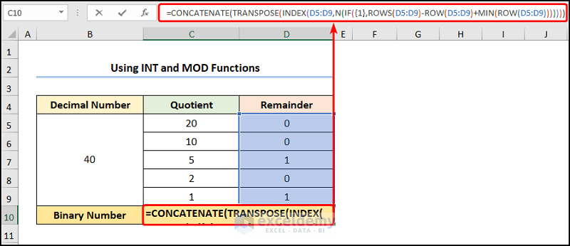
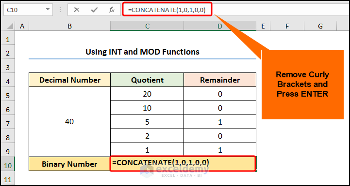
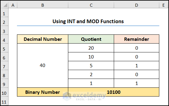
- Go to C10.
- Copy and paste the expression in the Formula Bar.
=CONCATENATE(TRANSPOSE(INDEX(D5:D9,N(IF({1},ROWS(D5:D9)-ROW(D5:D9)+MIN(ROW(D5:D9)))))))
Formula Breakdown:
- ROW(D5:D9) → the ROW function returns the row number of a reference. Here, D5:D9 points to the reference argument.
- Output → {5;6;7;8;9}
- MIN(ROW(D5:D9)) → the MIN function returns the smallest number in the {5;6;7;8;9} range: 5.
- Output → 5
- ROWS(D5:D9)-ROW(D5:D9)+MIN(ROW(D5:D9))
- 5 – {5;6;7;8;9} + 5 → {5;4;3;2;1}
- IF({1},ROWS(D5:D9)-ROW(D5:D9)+MIN(ROW(D5:D9))) → the IF function checks whether a condition is met. Here, {1} is the logical_test argument which represents TRUE. The function returns the value_if_false argument: ROWS(D5:D9)-ROW(D5:D9)+MIN(ROW(D5:D9)).
- Output → {5;4;3;2;1}
- INDEX(D5:D9,N(IF({1},ROWS(D5:D9)-ROW(D5:D9)+MIN(ROW(D5:D9))))) → the INDEX function returns a value at the intersection of a row and column in a given range. D5:D9 is the array argument, and N(IF({1},ROWS(D5:D9)-ROW(D5:D9)+MIN(ROW(D5:D9)))) is the row_num argument that indicates the row location.
- Output → {1;1;0;0;1}
- TRANSPOSE(INDEX(D5:D9,N(IF({1},ROWS(D5:D9)-ROW(D5:D9)+MIN(ROW(D5:D9)))))) → the TRANSPOSE function converts a vertical range of cells to a horizontal range. Here, INDEX(D5:D9,N(IF({1},ROWS(D5:D9)-ROW(D5:D9)+MIN(ROW(D5:D9))))) is the array argument.
- Output → {1,1,0,0,1}
- CONCATENATE(TRANSPOSE(INDEX(D5:D9,N(IF({1},ROWS(D5:D9)-ROW(D5:D9)+MIN(ROW(D5:D9))))))) → the CONCATENATE function joins several strings.
- Output → {“1″,”1″,”0″,”0″,”1”}
- Select the highlighted part of the formula.
- Press F9.
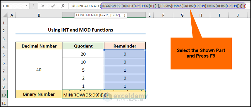
This is the output.
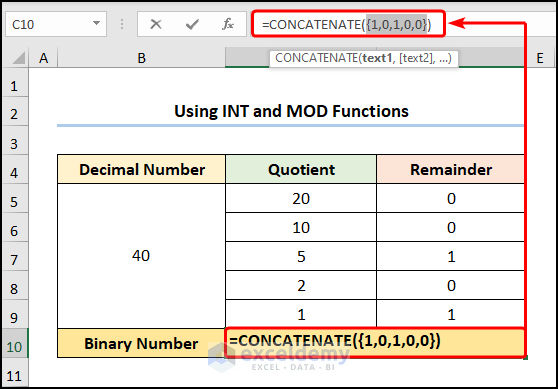
- Remove the curly brackets.
- Press ENTER.
Observe the GIF below.
This is the final output:
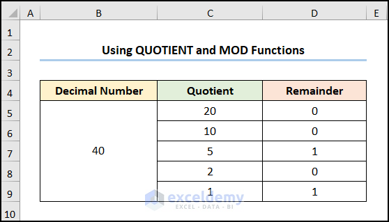
Method 3 – Using the Quotient and the MOD Functions
Steps:
- Follow the steps shown in the previous method. Instead of the INT function, use the QUOTIENT function.
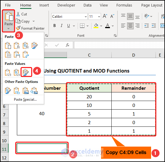
- Copy C4:D9.
- Move the cursor to B11.
- Click Paste.
- Choose Values & Source Formatting.
- Select B12:C16.
- Go to the Data tab >> click Sort >> in Sort by, choose Quotient >> select Smallest to Largest Order.
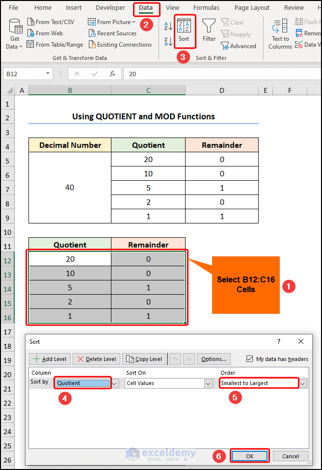
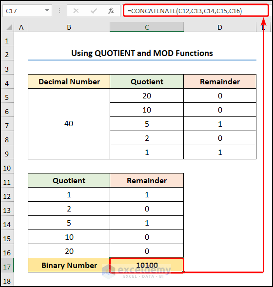
- Enter the formula below in C17.
=CONCATENATE(C13,C14,C15,C16,C17)
In the above formula, C13, C14, C15, C16, and C17 represent the sorted “Remainder” values.
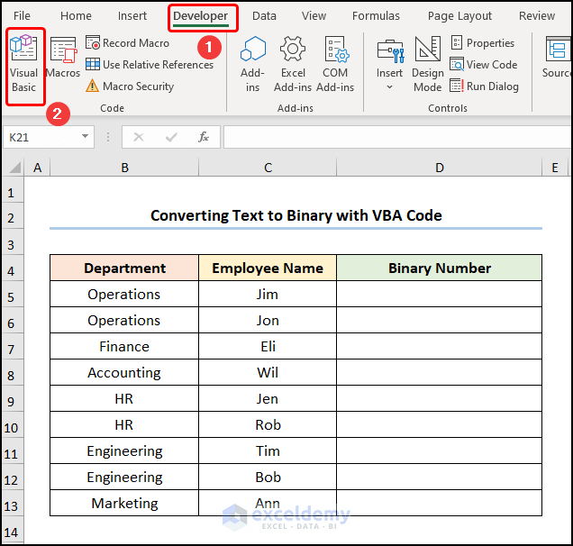
How to Convert Text to Binary in Excel
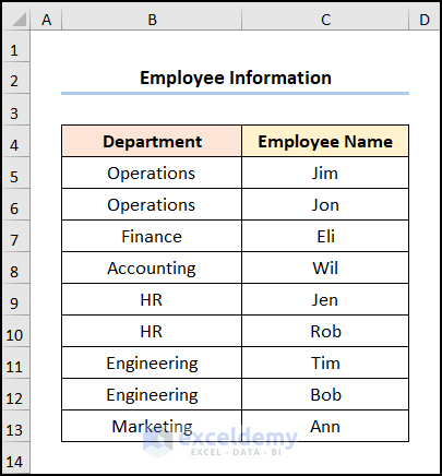
Convert the “Employee Names” into binary numbers:
Steps:
- Go to the Developer tab >> click Visual Basic.
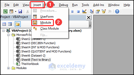
In the Visual Basic Editor:
- Select Insert >> choose Module.
Copy the code and paste it into the window.
Public Function String_To_Binary(str As String) As String
    Dim j As Long, lng As Long

    lng = Len(str)
    With Application.WorksheetFunction
        For j = 1 To lng
            String_To_Binary = String_To_Binary & .Dec2Bin(Asc(Mid(str, j, 1)))
        Next j
    End With
End Function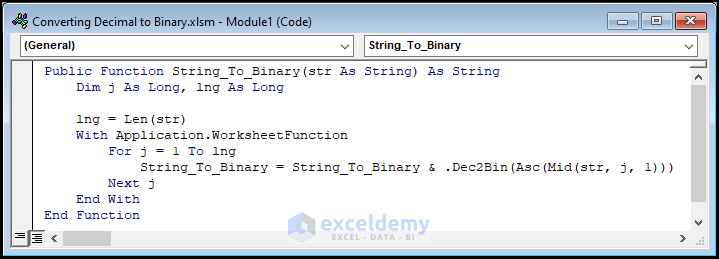
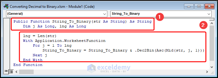
Code Breakdown:
- The function is given a name, here String_To_Binary().
- Define the variables j and lng and assign the data type: Long.
- Use the Len function to determine the length of the argument.
- Use the For Loop to loop through each text in the string and use the DEC2BIN and MID functions to convert the text to binary numbers.
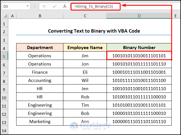
- Go to D5 >> use the function:
=String_To_Binary(C5)
C5 indicates the “Employee Name Jim”.
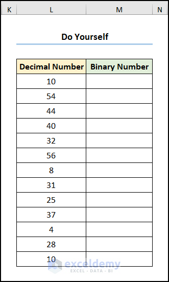
Practice Section
Practice here.
Download Practice Workbook
<< Go Back to | Excel Number System Conversion | Excel for Math | Learn Excel
Get FREE Advanced Excel Exercises with Solutions!
