Latest Posts From Afia Kona

Example 1 - Using ISODD Function to Sort Odd and Even Numbers in Excel We have added a Helper Column in the dataset where we will use the ISODD function. ...
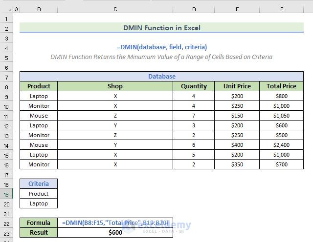
In many situations, we need to use the DMIN function to find the minimum value in a range of cells based on criteria. In the following article, we will ...
The dataset showcases Name, Salary, Week, and Per Week Salary. To determine per week salary by dividing Salary by Week: Use the following formula in ...
The following dataset showcases vector data: Data A and Data B. Example 1 - Using an Addition Formula to Sum Two Vector Data Steps: ...
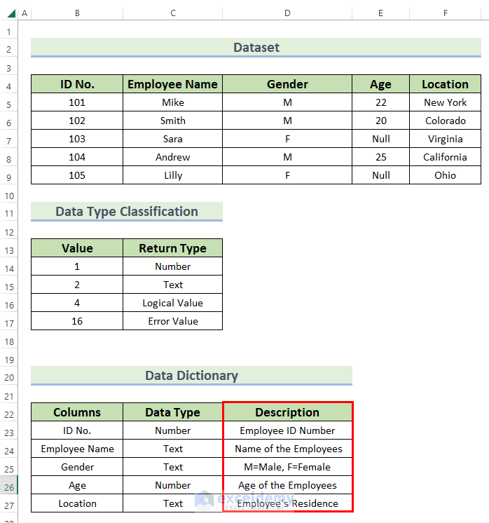
If you want to create a data dictionary in Excel, you have come to the right place. Here, we will walk you through 3 easy steps to do the task smoothly. ...
Step 1 - Creating a Dataset for the Workflow Tracker We have listed the tasks in the Task column. Input the starting dates in the Starting Date ...

Here are 10 simple ways to navigate between sheets in Excel: Method 1 - Clicking on the Sheet Name Tab Simply click on the desired sheet name tab, e.g. ...

In the following dataset, you can see the Product and Supply Date columns. We have several Supply Dates that include dates both in the future and the ...

In this article, we will demonstrate how to insert and rotate a spin button in Excel to change a value. What Is a Spin Button? A Spin Button is a form ...

If you want to edit tooltip in Excel, you have come to the right way. Here, we will walk you through 2 easy methods to do the task smoothly. What Is ...
If you want to create 3D animation in Excel, you have come to the right place. Here we will walk you through 2 easy methods to do the task smoothly. How ...

Linear optimization is one of the key topics of statistics. We can perform predictive analysis using the variables' available data. In the following article, ...
What Is Excel VBA TextBox? In Excel VBA, a TextBox is a user interface element that allows users to input data. The sample worksheet Student List ...
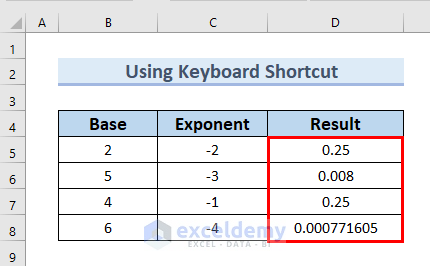
In the following dataset, you can see the Base and Exponent columns. The Exponent column has negative exponents. Method 1 - Using Keyboard Shortcuts ...

An Overview of an Audit Checklist In the following picture, you can see an overview of an Audit Checklist. We will show you how you can create such an ...
- « Previous Page
- 1
- 2
- 3
- 4
- …
- 10
- Next Page »
See Our Reviews at


Hello Mark W
I hope after reading my reply, you will be able to solve the problem.
1. First, let me explain to you how the TRIM function works.
Suppose, you have the name “ Joe Louis “, and you can see this name has leading, middle, and trailing spaces. In that case, the TRIM function will work.
The result will be like “Joe Louis”.
However, if the name is like “ Joe Lou is “, the TRIM function will only remove the leading and trailing space of the name. It will not remove the space between letters.
The final result of the above name will be “Joe Lou is”.
Now, suppose you have a number like “ 12 24 5 6 “, in this case, the TRIM function will only remove the leading and trailing spaces. Therefore, after applying the TRIM function.
The number will look like “12 23 5 6”.
I hope that now you will easily understand in which situations, the TRIM function works.
2. After that, let me explain to you how the SUBSTITUTE function works.
If you have a number like “ 1 2 45 7 “ then the SUBSTITUTE function will eliminate all the spaces. Here, suppose the old number is in cell C4. Therefore, you have to type =SUBSTITUTE(C4,” “,””).
After that, the number will become like “12457”.
Next, if you have a word where the letters have spaces between them like if you have “ Yell ow “ in a cell, the SUBSTITUTE function will remove the spaces. Here, suppose the old number is in cell C4. Therefore, you have to type =SUBSTITUTE(C4,” “,””).
The result will be “Yellow”.
However, if a Text has spaces between words then we have to identify and add the space in the SUBSTITUTE function properly. Let’s say, the name “ Adam Smith “ is present in cell C4. You can easily notice that there are three spaces between Adam and Smith. Along with that, there are lading and trailing spaces. we have to type =SUBSTITUTE(F16,” “,” “), here you to give three spaces in between the first double quote. Along with that, make sure to keep one space between the second double quote, otherwise both the words will merge into one word.
The outcome will be “Adam Smith”
I hope that when using the SUBSTITUTE function if you can identify the spaces between words, and add the space properly in the formula, your problem will be solved.
3. Let us now discuss how Find and Replace works.
Find and Replace is a useful feature to replace spaces between numbers in a cell. If you want to replace spaces between numbers, Find and Replace is an effective and easy way.
However, For different numbers of spaces between words, we have to identify those spaces, and in the Find what box we need to press those Exact numbers of spaces. Otherwise, the Find and Replace will not work. Therefore, if different numbers of spaces between text are present in different cells then the cells need a unique number of spaces in the Find what box.
I hope you can identify the spaces between words, and in the Find what box you can press exactly the same number of spaces. Hence, your problem might be solved.
4. When different cell content has a different number of spaces, Power Query is extensively useful to remove those spaces.
As in your comment, you did not mention anything regarding Power Query, I highly suggest you use Power Query. I am hopeful that it will solve your problem.
Thank you for your comment. I hope you will now be able to solve your problem. If, however, these methods still do not work for you, please share your Excel file in the comment section. This will help me to understand the problem, and I will try my best to solve the problem.
Regards!
Dear Tanzir,
Thank you for your comment.
Arcsine transform is done for real numbers ranging from 0 to 1.
In the formula, DEGREES(ASIN(SQRT(X/100))), X indicates the percent value to be transformed. Therefore, when we put 50% in the formula it actually becomes 0.5. As a result, we can Arcsine transform the data.
However, if we put 50 instead of 50% then Arcsine transform is not possible.
Regards
Afia Aziz Kona
Dear Kristian,
Thank you for your comment.
You can solve your problem by using one of the following procedures:
1. Using Document Inspector Command
2. Editing Trust Center for External Content
3. Inputting Accurate Data Importing File Destination
4. Setting Refreshing Option in Beginning
5. Installing an Updated Version of Excel
You can read the following two articles to get descriptive information.
https://www.exceldemy.com/excel-external-data-connections-have-been-disabled/
https://www.exceldemy.com/excel-data-connection-not-refreshing/
I hope your problem will be solved.
Best,
Afia Aziz Kona
Dear Sam,
Thank you for your comment. I understand that you are looking for a more dynamic Attendance Sheet, if so, you can use the following VBA code as an update:
Download this Excel file for a better understanding.
I hope that your problem will be solved now. If you have any further issue, please let us know in the comment section.
Best
Afia Aziz Kona
Excel and VBA Content Developer
Exceldemy
Dear DEREK TIERNEY,
Thank you for your comment.
After typing the code for the Command Button in Step 8, you have to call the private sub Call D_Display in the previous code. This will solve the problem. If you still face the issue, please attach the Excel file in the comment section.
Best,
Afia Aziz Kona
Dear CONCERNEDEXCELUSER,
Thank you for your comment.
Please have a look at the graph, the error bar for Study 6 is at the topmost position. And point 1.88 is right next to point 1.84.
Thank you.
Regard,
Afia Aziz Kona
Content Developer
Exceldemy
Dear NICK,
Thank you for your comment. Please follow the second method, Using Format Data Series Option. For a Combo Chart, this method will work.
I hope your problem will be solved now. If, however, you are still facing an issue, you can send us your Excel file to [email protected].
Best,
Afia Aziz Kona
Excel & VBA Content Developer
Exceldemy
Dear Damien,
Thank you for your comment. To get “zero” or “Nil” for the value 0, you have to simply add an IF statement with the code.
you can use the following code:
Best,
Afia Aziz Kona
Dear Wietze,
Thank you for your comment. unfortunately, your question seems unclear to me. If you can provide me with your Excel file and be more specific about your inquiry, I will be able to help you. Please share your Excel file.
Best,
Afia Aziz Kona
Dear AAMIR
Thank you for your comment.
If you want to make a recorder for only half-day casual leave, you can use the same template in this article. In this case, each “1” will be a half-day leave. And the total will imply a total half day’s leave. Change the header for your needs.
Also, for better reach, you can review the following article to record a half-day casual leave.
https://www.exceldemy.com/calculate-half-day-leave-in-excel/
Best,
Afia Aziz Kona
Hello Chris,
Thank you for your comment.
The option, “Data >> Get Data >> From Other Sources >> From Microsoft Query” should be available in Excel 2019 since Power Query is available in Excel 2019.
However, since you are unable to find the option, I would suggest you to install a new version of Excel. I hope your problem will be solved now.
Best,
Afia Aziz Kona
Dear Deepak,
Thank you for your comment.
To show 100 in value 25=100/4, you need to apply the following Custom Cell Format.
Best,
Afia Aziz Kona
Dear Ella,
Thank you for your comment. I will try to provide a proper answer to your question.
The first answer is, to set the value for b0, b1, and b2, you can assume any values. Then, you can optimize the assumed values.
The answer to the second question is, since we have 2 independent and one dependent variable, we took 3 initial problem-solver variables. One for the dependent variable, and then for each independent variable, we took 1 additional problem solver variable.
I hope this will help you.
Regard,
Afia Aziz Kona
Dear Yos,
Walaikum’assalam. Thank you so much for your comment. I will try my best to give you a proper solution.
Firstly, I will show you how you can import a .pdf file to a .txt file, and after that, I will show you the VBA code to open the text file in Excel.
Let me show you how you can import a .pdf file to a .txt file.
● First of all, upload your PDF file to your Google Drive.
● Then, from Google Drive >> right-click on the uploaded PDF file.
● Then, click on Open With from the Context Menu >> select Google Docs.
This will open the PDF as a Google Doc file.
● After that, go to the File tab of Google Docs >> click on Download.
● This will bring out several Download options >> select Plain Text (.txt)
This will make the Google Docs as a Text file.
● Next, open your Text file and see the outcome.
Next, I will show you how you can open the Text file in Excel using VBA.
In the beginning, carefully notice the location of the Text file, and also carefully note the name of the file.
Here, we have marked our text file name.
This is because we have to implement the file name and location in the VBA code properly.
Now, it is time to open a VBA Module.
● To open a VBA module, open your Excel file >> go to the Developer tab >> select Visual Basic.
You can also press the ALT+F11 keys.
This will open a VBA Editor window.
● Furthermore, from the Insert tab >> select Module.
● Moreover, in the Module, type the following code.
Here, change the location and name of the text file according to your file.
● Afterward, Save the code >> Run the code.
Therefore, you will see the Excel file will have all the texas.
I hope this was helpful. Please let us know if you have any additional queries.
Regard,
Afia Aziz Kona
Dear W
Thank you for your comment.
Let me show you that your formula works properly.
Here, I created the List column including cells F2:F4.
Along with that, I created a Product column that includes cell J2.
Here, as I do not know your actual dataset, I take List and Product according to my choices, however, the cells are the same as your description.
Further, I type the following formula in cell B4.
=TEXTJOIN(", ", TRUE, IF(COUNTIF(J2,"*"&$F$2:$F$4&"*"), $F$2:$F$4, ""))This is the same formula you mentioned in the comment.
After that, I press ENTER.
As a result, you can see the result in cell B4.
Therefore, the formula works properly.
I hope that your problem will be solved now.
If you face any further problems, please share your Excel file with us in the comment section.
Regards
Afia Aziz Kona
Dear ABBY SHULER
Thank you for your comment. Here, for your first problem, to get rid of the #NAME error, you can copy the following VBA code in a new Excel Workbook. The uploaded Excel file sometimes show problem while running on a different computer, therefore, when you will copy the code to a new workbook, the #NAME error will be solved.
Function AddressCompare(first_string As String, Second_string As String, _
Comparing_Letters As Integer) As Double
Dim int_character As Integer, Comparing_LettersMatch As Integer
Dim n_Gram_List1 As String, n_Gram_List2 As String, n_letter_Gram As Variant
Dim n_Gram_array1 As Variant
For int_character = 1 To Len(first_string) – (Comparing_Letters – 1)
If n_Gram_List1 <> “” Then n_Gram_List1 = n_Gram_List1 & “,”
n_Gram_List1 = n_Gram_List1 & Mid(first_string, int_character, Comparing_Letters)
Next int_character
For int_character = 1 To Len(Second_string) – (Comparing_Letters – 1)
If n_Gram_List2 <> “” Then n_Gram_List2 = n_Gram_List2 & “,”
n_Gram_List2 = n_Gram_List2 & Mid(Second_string, int_character, Comparing_Letters)
Next int_character
n_Gram_array1 = Split(n_Gram_List1, “,”)
For Each n_letter_Gram In n_Gram_array1
If InStr(1, n_Gram_List2, n_letter_Gram) Then
Comparing_LettersMatch = Comparing_LettersMatch + 1
End If
Next n_letter_Gram
AddressCompare = Comparing_LettersMatch / (UBound(n_Gram_array1) + 1)
End Function
After that, save the code and go back to your worksheet. I hope the #NAME error will be gone now.
For your second query, you can use 3 instead of 2. Using 3 will compare 3 letters at a time, and therefore, the result will decrease the match percentage between two addresses.
When you will use 2, it will compare 2 letters at a time, and therefore, the match percentage between two addresses will be higher.
Let me show you that elaborately.
When we use
=AddressCompare(C5, F5, 2)in cell E3, the result becomes 1, which indicates the Exact Match.However, the two addresses are not the same, therefore, using 2 does not give an accurate result.
On the other hand, when we use the formula
=AddressCompare(C5, F5, 3)in cell E3, the result becomes 0.970588235, which does not indicate the Exact Match. Rather, it suggests that there is some dissimilarity between the two addresses.Therefore, using 3 is wise in your case.
Here, another thing must be noted, for your address match, you have to set your own creation while using the IF function.
Let me elaborate on this.
Here, in cell F3, we type the following formula.
IF(AddressCompare(C5, F5, 3)>0.5, "Full Match", "No Match")Here, in this formula, we give the criteria, that when AddressCompare(C5, F5, 2) is greater than 0.5, the IF function returns “Full Match“. However, when AddressCompare(C5, F5, 2) is not greater than 0.5, the IF function returns “No Match“.
Therefore, in cell F3 the result is “Full Match“.
However, there is some dissimilarity between the two addresses. Hence, the result in cell F3 is not accurate.
To get an accurate result, we will type the following formula in cell F3.
IF(AddressCompare(C5, F5, 3)>0.99, "Full Match", "No Match")Here, in this formula, we give the criteria, that when AddressCompare(C5, F5, 2) is greater than 0.99, the IF function returns “Full Match“. However, when AddressCompare(C5, F5, 2) is not greater than 0.99, the IF function returns “No Match“.
Therefore, in cell F3 the result is “No Match“.
This is the correct result.
I really hope that you get your answer, and that you can solve your problems.
If you face any problem, you can always let us know.
Regards,
Afia Aziz Kona
Dear Ashiliah
Thank you for your comment.
Let me now show you how you can solve your problem.
Based on your description I’ve created the dataset.
Here, you can see in the following picture that we have Chocolate lava Cake in cell A5. we keep this in Sheet1.
After that, in Sheet2, we have Lava cake, Strawberry drink, and Banana muffin in cells A5, A6, and A7 respectively.
Next, we will type the following formula in cell B5 of Sheet1.
=TEXTJOIN(", ", TRUE, IF(COUNTIF(A5, ""&Sheet2!A5:A6&""),Sheet2!A5:A6, ""))After that, press ENTER.
As a result, you can see Lava cake in column B of sheet1.
I hope you understand the solution. If you have any problems you can always let us know in the comment section.
Regard
Afia Aziz kona
Dear Jacob Smith
Thank you for your comment.
The first method works properly when you press the SHIFT key after selecting rows/columns.
Let me explain this elaborately.
Here, in the following dataset, we want to move rows 7 and 8.
To do so, first, we will select cells B7:D8.
After that, we will hover our mouse cursor to the edge of the selection and wait for it to change into a 4 directional cross.
At this point, press the SHIFT key.
Along with that, left-click on it with your mouse and drag your selection to the desired location.
A green line should appear to assist you to drop it at the desired location.
Here, we drag the selected rows to Row 3, and therefore, you can see a Green Line at Row 3.
In addition, you can see B4:D5 on the left side of the Green line which indicates the final location of the selected rows.
After that, we will release the mouse and SHIFT key.
As a result, you can see the movement of rows to a new location.
I hope that you can now use Method-1.
If you have any problems, you can always let us know in the comment section.
Regard
Afia Aziz Kona