
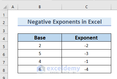
In the following dataset, you can see the Base and Exponent columns. The Exponent column has negative exponents.
Method 1 – Using Keyboard Shortcuts to Use Negative Exponents in Excel
Steps:
- Enter the following formula in D5.
=B5^C5After =B5, use SHIFT+6 to display ^ and enter C5.
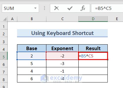
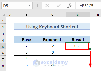
- Press ENTER.
You can see the result in D5.
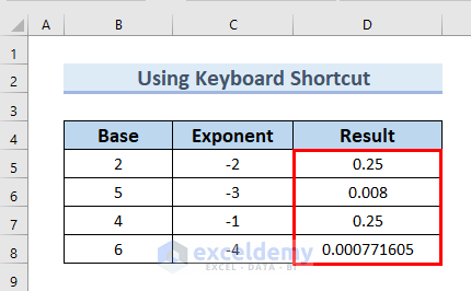
- Drag down the Fill Handle to see the result in the rest of the cells.
This is the output.
Method 2 – Using the POWER Function in Excel
Steps:
- Enter the following formula in D5.
=POWER(B5,C5)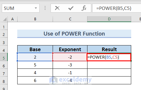
Formula Breakdown
- POWER(B5,C5) → returns the outcome of a number raised to a power.
- B5 →is the number.
- C5 → is the power.
- Outcome: 0.25
25 is the result of 2 raised to -2.
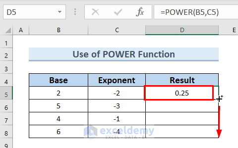
- Press ENTER.
You can see the result in D5.
- Drag down the Fill Handle to see the result in the rest of the cells.
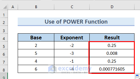
This is the output.
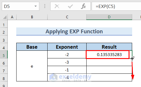
Method 3 – Applying the EXP Function to use Negative Exponents
Find the negative exponent of base e:
Steps:
- Enter the following formula in D5.
=EXP(C5)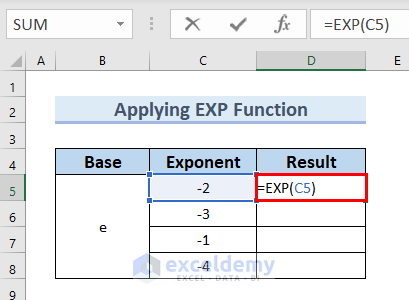
Formula Breakdown
- EXP(C5) → returns e (Euler’s Number) raised to the power of number.
- C5 → is the number
- Output: 0.135335283
- Press ENTER.
You can see the result in D5.
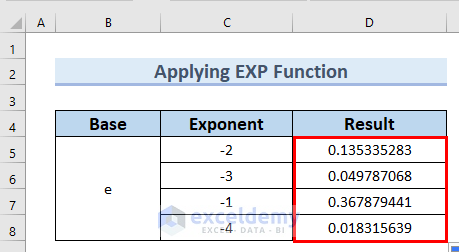
- Drag down the Fill Handle to see the result in the rest of the cells.
This is the output.
Read More: How to Use Excel Exponential Function of Base 10
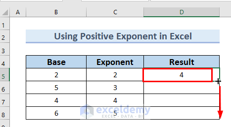
How to Use Positive Exponents in Excel
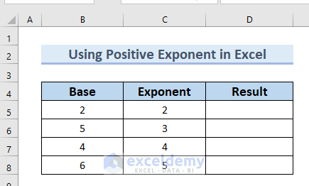
Steps:
- Enter the following formula in D5.
=POWER(B5,C5)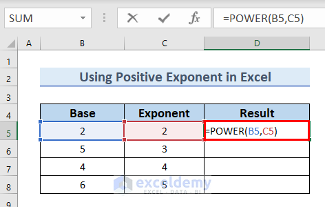
Formula Breakdown
- POWER(B5,C5) → The POWER function returns the outcome of a number raised to a power.
- B5 →is the number.
- C5 → is the power.
- Outcome: 4
4 is the result of 2 raised to 2.
- Press ENTER.
You can see the result in D5.
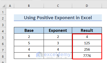
- Drag down the Fill Handle to see the result in the rest of the cells.
This is the output.
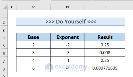
Practice Section
Practice here.
Download Practice Workbook
Download the Excel file.
Related Articles
- How to Type Exponential in Excel
- Convert Scientific Notation to x10 to the Power of 3 in Excel
- How to Estimate Inverse Exponential in Excel
- How to Use Exponent Symbol in Excel
- How to Display Exponents in Excel
<< Go Back to Excel EXP Function | Excel Functions | Learn Excel
Get FREE Advanced Excel Exercises with Solutions!
