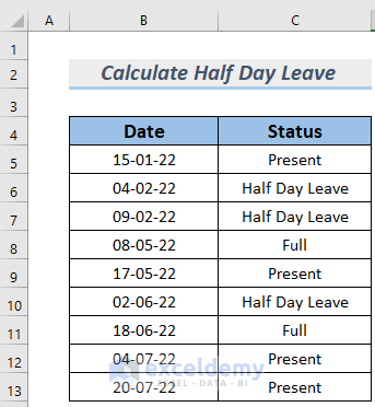
In the dataset, we have the attendance statuses of an employee in a period.
Method 1 – Using Excel COUNTIF Function to Calculate Half Day Leave
Steps:
- Select a cell to store the number of half day leaves and type the following formula in it:
=SUM(COUNTIF(C5:C10,{"Present","Full Day Leave","Half Day Leave"})*{0,0,0.5})
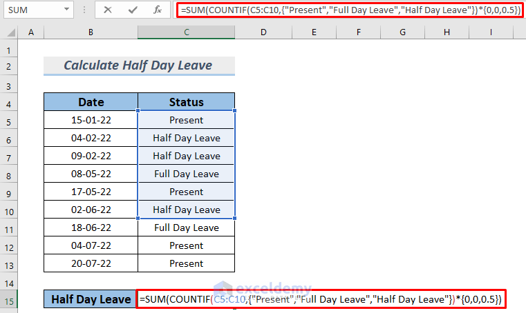
Here, we are using an array formula to count both “Present” and “Full Day Leave” as 0 (zeros) and “Half Day Leave” as 0.5. The COUNTIF function will count the number of each category ( “Present”, ”Full Day Leave”, and “Half Day Leave”) and will return an array containing the number of the types. This will be multiplied by the {0,0,0.5} array. The SUM function then sums up all the half-day leaves and returns that value.
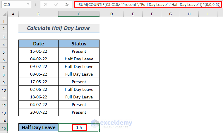
- Press the Enter button and you will see the number of half-day leaves in cell C15.
Method 2 – Implementing Combined Formula to Calculate Half Day Leave
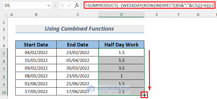
Suppose that employees work half of the day on Friday. So, we should count Friday as a half-working day.
Steps:
- Make a column to store half days and type the following formula in it:
=SUMPRODUCT(--(WEEKDAY(ROW(INDIRECT(B5&":"&C5)))=6))/2
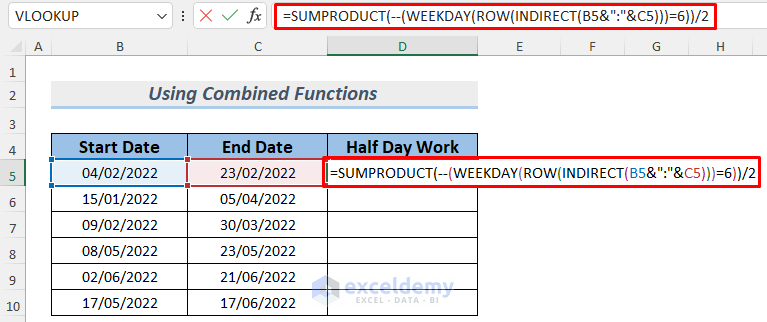
The formula uses SUMPRODUCT, WEEKDAY, ROW and INDIRECT functions.
Formula Breakdown
- INDIRECT(B5&”:”&C5) —-> returns an array that has a row number the same as the date in cell C5 converted to its number
- ROW(INDIRECT(B5&”:”&C5)) —-> turns into an array of dates (in number format) from the 4th February to the 23rd February.
- Output: {44596;44597;44598;44599;44600;44601;44602;44603;44604;44605;44606;44607;44608;44609;44610;44611;44612;44613;44614;44615}
- WEEKDAY(ROW(INDIRECT(B5&”:”&C5))) —-> returns an array of weekdays in number from the 4th February to the 23rd February.
- Output: {6;7;1;2;3;4;5;6;7;1;2;3;4;5;6;7;1;2;3;4}
- –(WEEKDAY(ROW(INDIRECT(B5&”:”&C5)))=6) —-> will become the following array where the 6th day of the week will be noted as 1 and others as 0.
- Output: {1;0;0;0;0;0;0;1;0;0;0;0;0;0;1;0;0;0;0;0}
- SUMPRODUCT(–(WEEKDAY(ROW(INDIRECT(B5&”:”&C5)))=6))/2 —-> turns into the summation of half days.
- Output: 1.5
- Hit Enter to get the number of half working days in cell D5 from the 4th February to the 23rd February.

- Use the Fill Handle to AutoFill the lower cells.
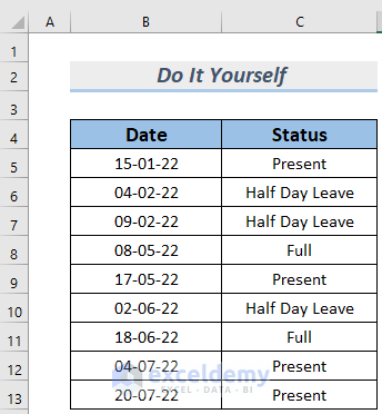
Practice Section
Here’s the dataset of this article so that you can practice these methods on your own.
Download Practice Workbook
<< Go Back to Leave Calculation | Formula List | Learn Excel
Get FREE Advanced Excel Exercises with Solutions!
