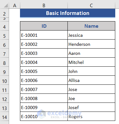
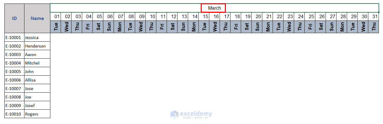
Step 1 – Insert Employee Information
We are going to calculate the annual leaves of an organization consisting of 10 employees.
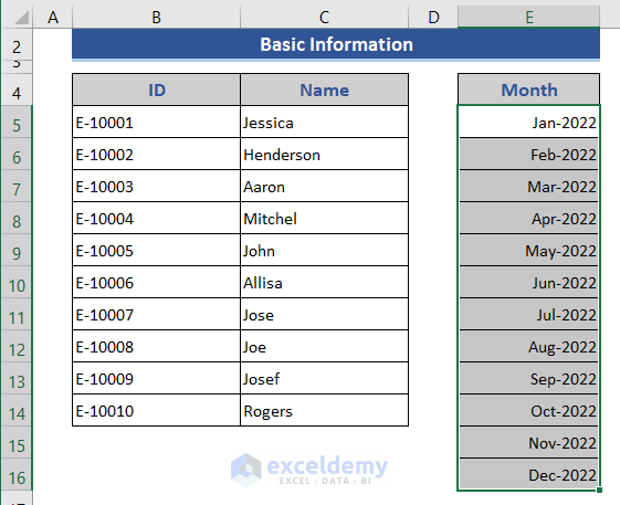
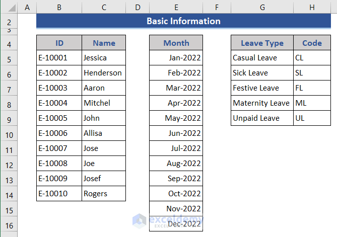
- Input the Names and IDs of employees.
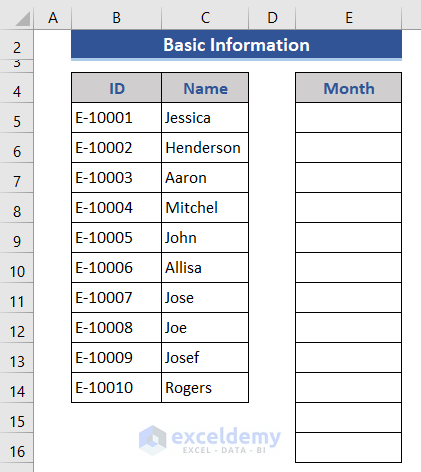
Step 2 – Create a List of Leaves Allowed by Company
- Input the names of months in a separate column.
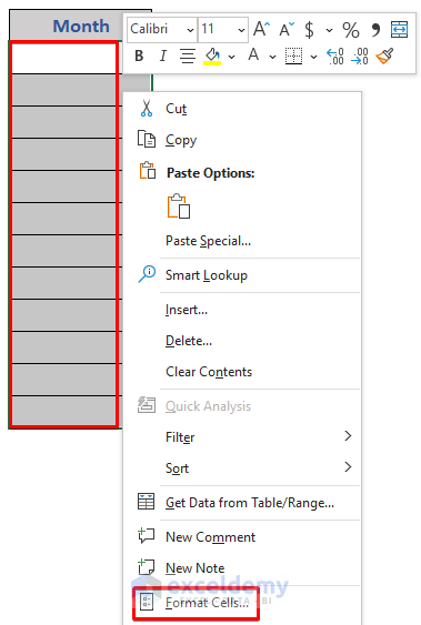
- Select all the cells of the Month column.
- Right-click and select the Format Cells option.
- Click on the Number tab.
- Choose a date Type from the Custom field.
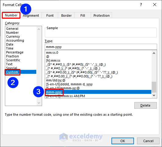
- Press the OK button.
- Add a list of leaves with their codewords.
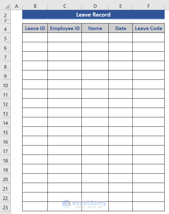
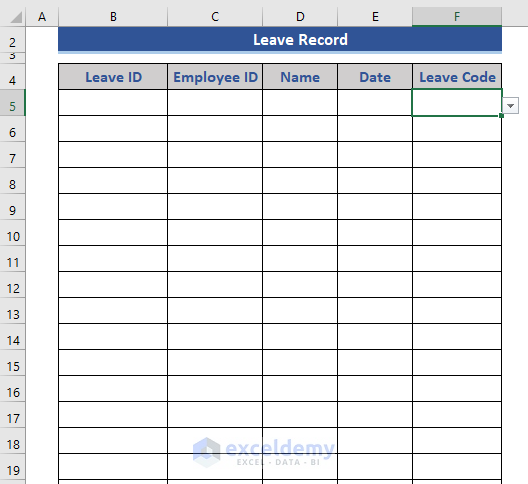
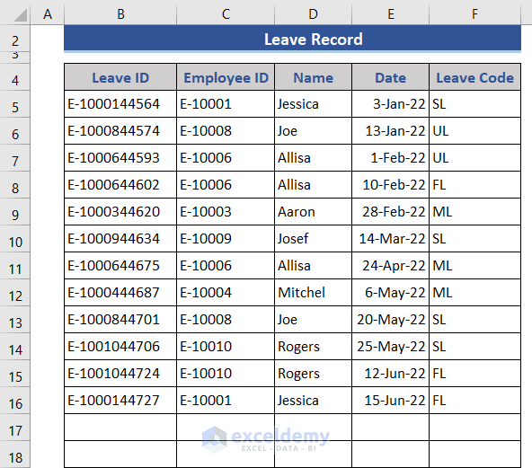
Step 3 – Create a Leave Record
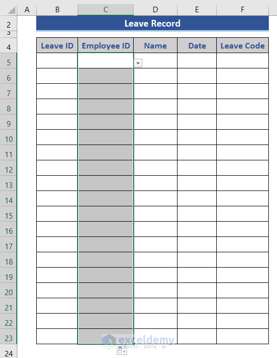
- Create a worksheet with the following columns: Leave ID, Employee ID, Name, Date, Leave Code.
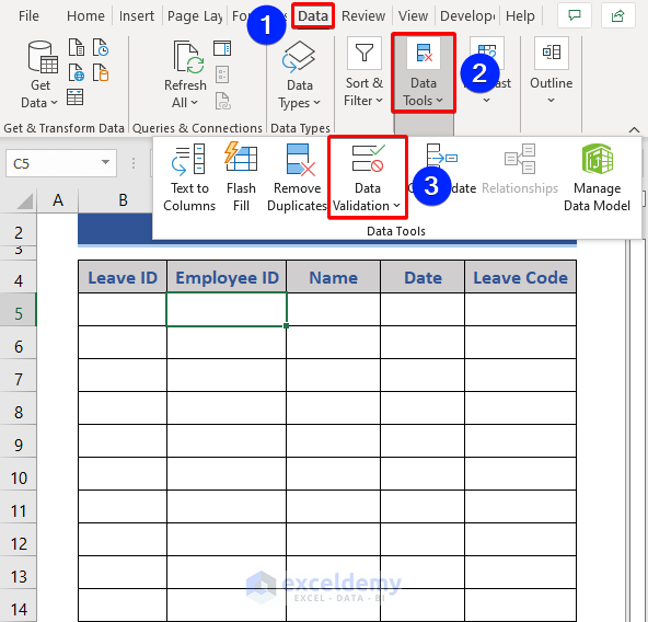
- Click on Cell C5.
- Go to the Data tab.
- Click on the Data Validation option from the Data Tools group.
- The Data Validation window appears here.
- Choose List in the Allow box.
- The source sheet is the basic information. Choose the Employee ID cells here.
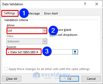
- Press the OK button.
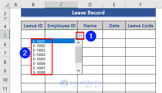
- Extend the Data Validation to all the cells of that column.
- Click on the Drop-down button and see the options.
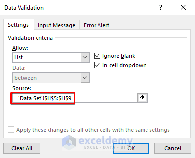
- Apply data validation for the Leave Code column.
- The source is the cells of the leave types.
- Data Validation was successfully applied for both columns.
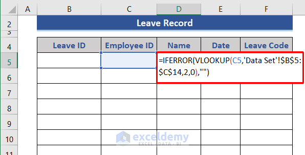
- Apply the following formula to Cell D5.
=IFERROR(VLOOKUP(C5,'Data Set'!B5:C14,2,FALSE),"")
- Apply the formula below to Cell B5.
=C5&E5
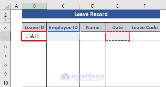
This forms a unique ID combining the Employee ID and Date value.
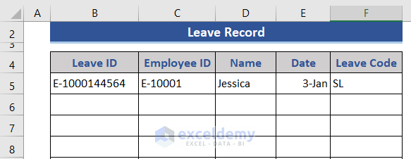
- Input leave information in the first row.
- Insert the leaves per your requirements.
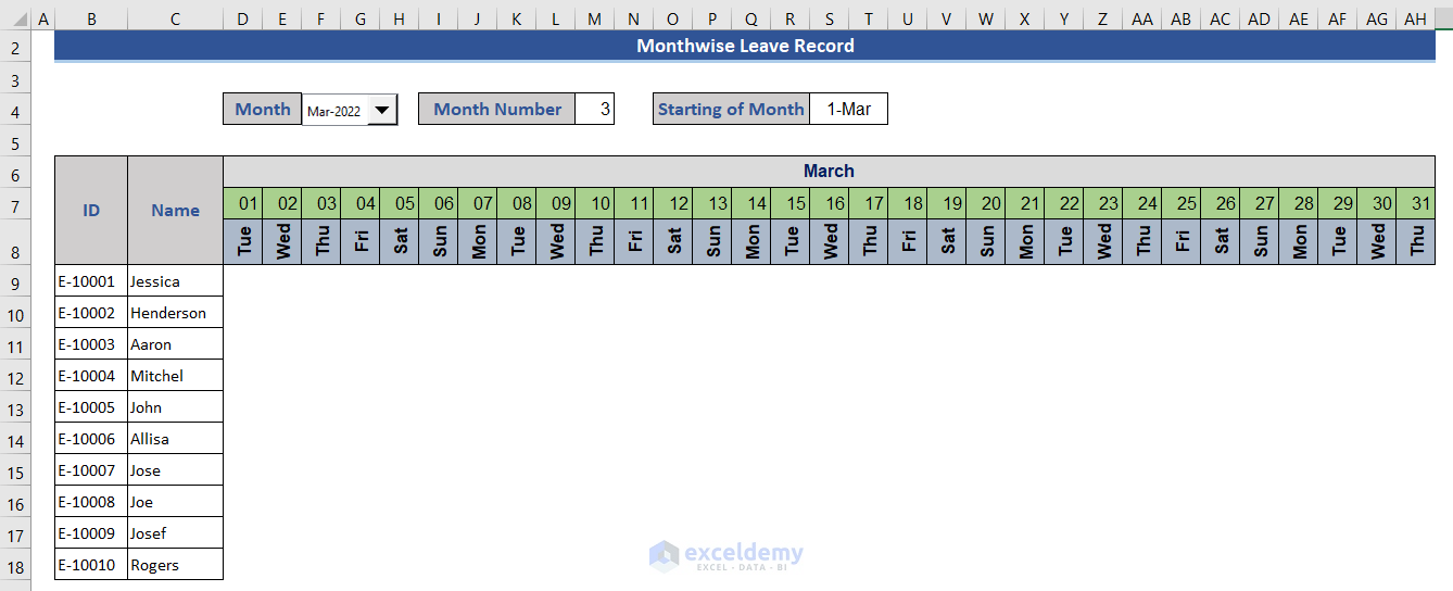
Step 4 – Calculate Monthly Leaves
- Click on the Developer tab.
- Choose Combo Box from the Insert group.
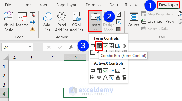
- Place the Control Box in a table.
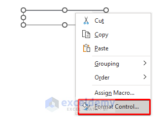
- Right-click on the Combo Box and select Format Control.
- Click on the Control tab.
- Select a range of month names at the Input range.
- Link a cell that will show the serial number of that month based on the source.
- For Drop down lines, put 12 because of 12 months of the year.
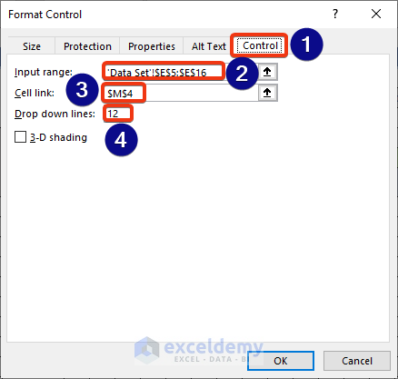
- Press OK.
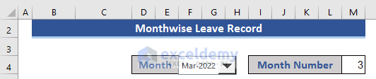
We can see the selected month from the drop-down and the corresponding month number.
- Use this formula on Cell S4.
=INDEX('Data Set'!E5:E16,'Monthly Leave Record'!M4)
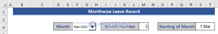
This will extract the starting date of the month the depending on month number.
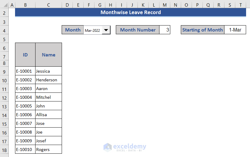
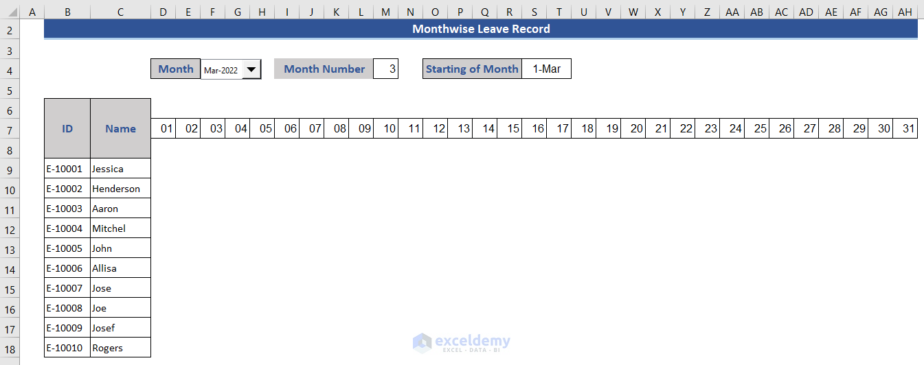
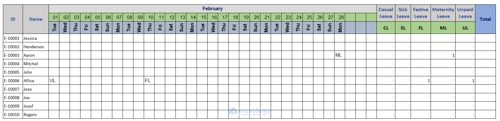
- Input the IDs and Names in the columns in the dataset.
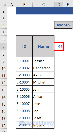
- Go to cell D7 and input S4.
- Go to cell E7 and put the following formula.
=IF(D7="","",IF(EOMONTH($S$4,0)<D7+1,"",D7+1))
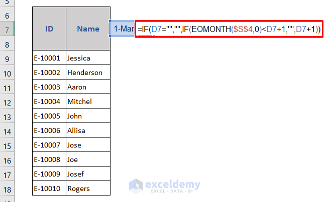
- Press the Enter button.
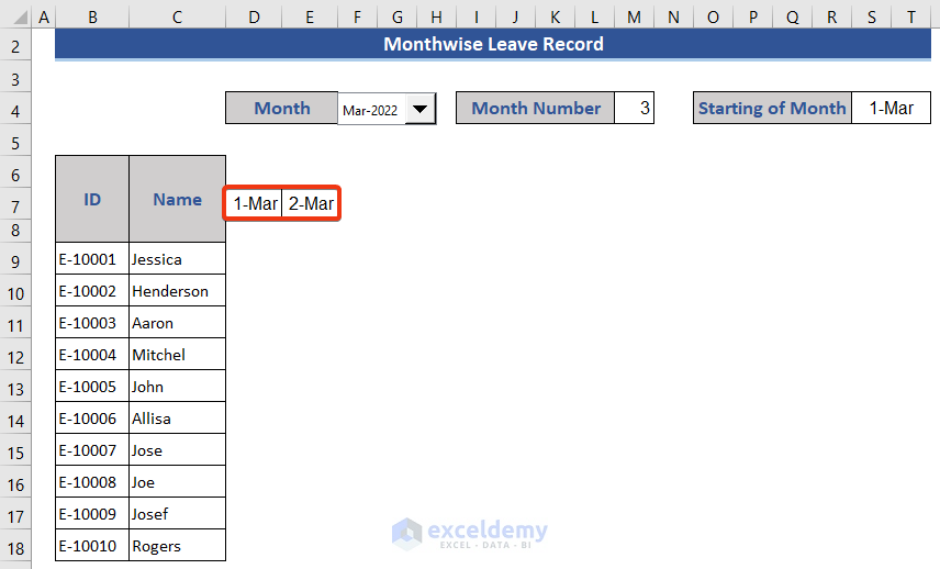
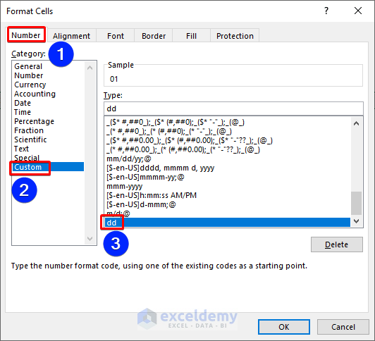
- Choose the format dd from the Custom options.
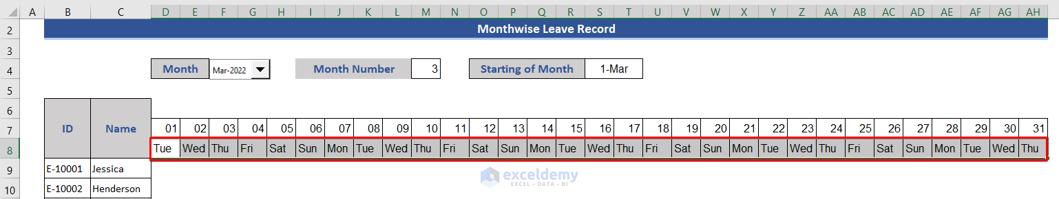
- Expand the cells to a total of 31 cells for 31 days of the month.
- Put the following formula in Cell D8.
=TEXT(D7,"ddd")
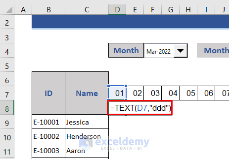
- Hit Enter and AutoFill that formula to the right to cover all days.
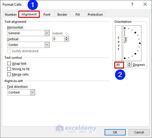
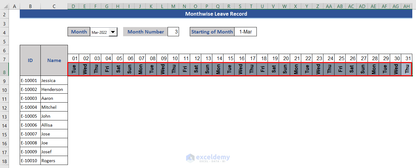
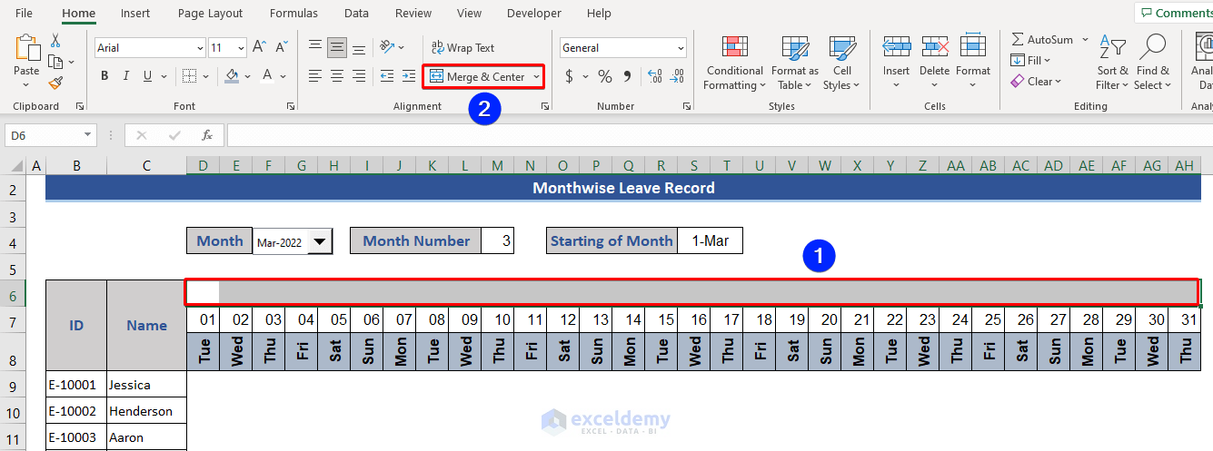
- Click the Alignment tab.
- Rotate 90 degrees.
- Look at the dataset.
- Select D6:AH6.
- Click on Merge & Center.
- Input S4 on that cell.
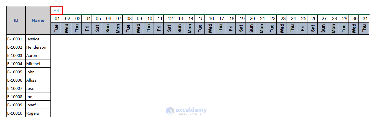
- Look at the worksheet.
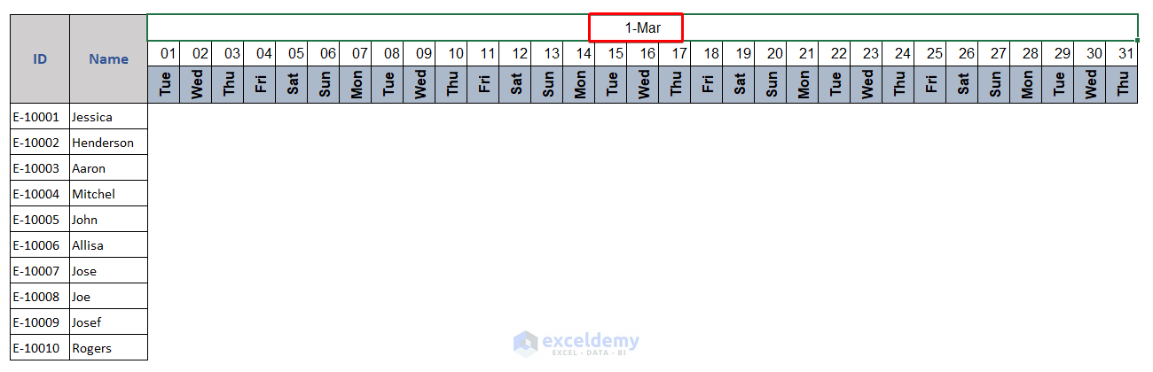
- Change the format of that cell to mmmm from the Format Cells window.
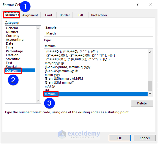
- Only the month name is showing now.
- Change the font and background color for the various table elements.
- Put the following formula in Cell D9.
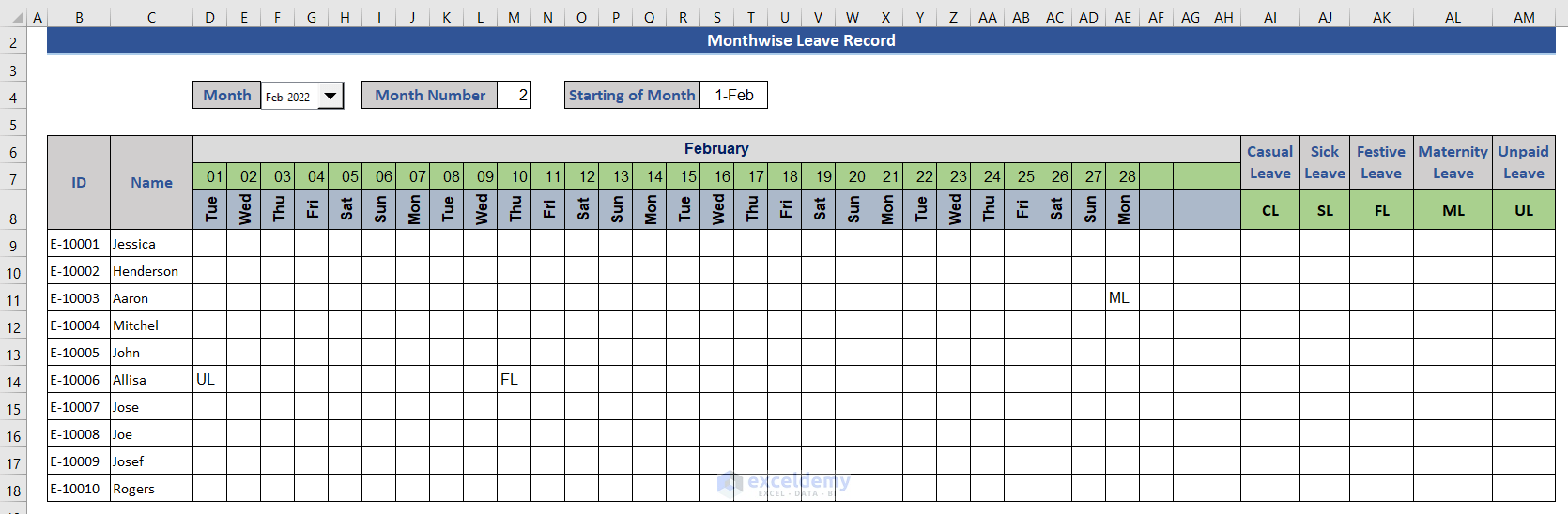
=IFERROR(VLOOKUP($B9&D$7,Record!$B:$F,5,FALSE),"")
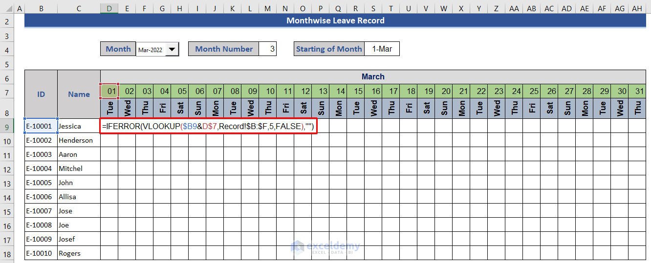
- Expand the formula to all the cells of the month section.
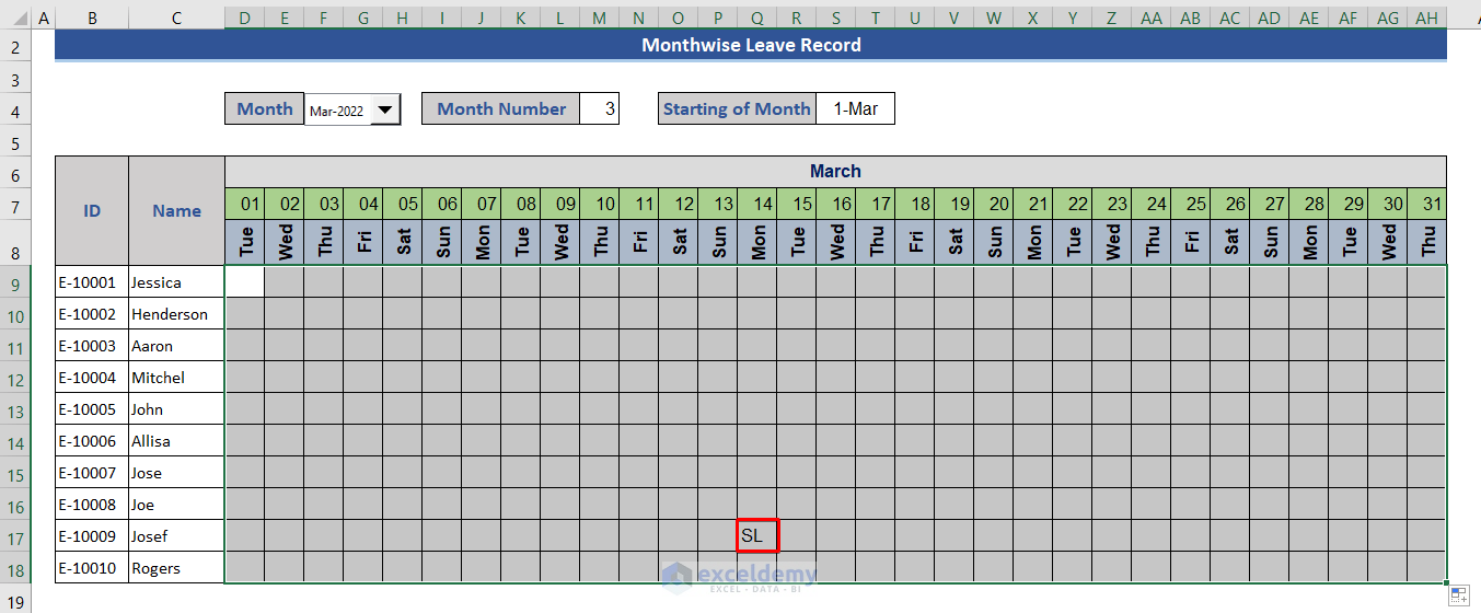
We can see leaves with corresponding codes showing.
- Change the month name from March to February.
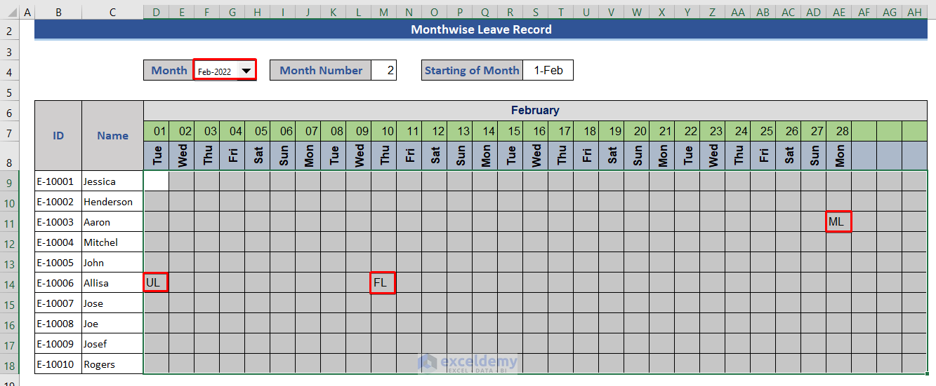
- Leave dates have changed successfully.
- Add 5 new columns with leave names and codes.
- Put the following formula in Cell AI19.
=COUNTIF($D9:$AE9,AI$8)
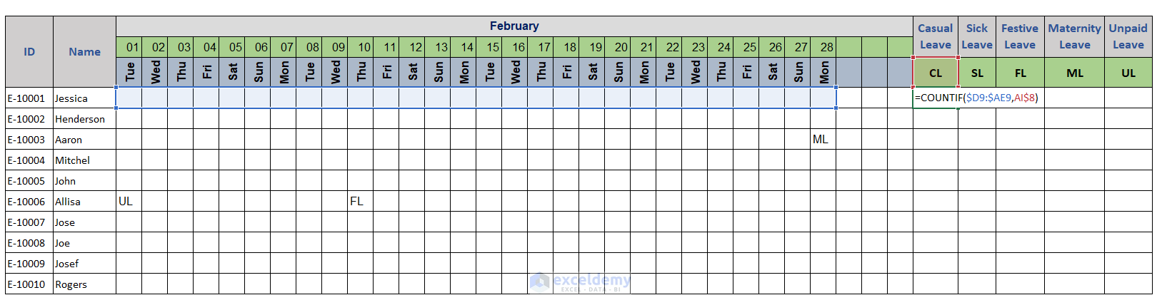
- Expand that formula to the rest of the cells.
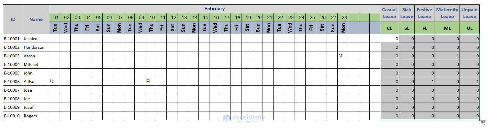
- Select AI9:AM18.
- Go to the Conditional Formatting group.
- Choose Equal To from Highlight Cells Rules.
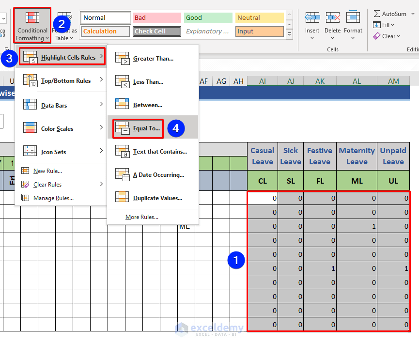
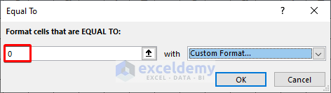
- Put 0 in the box and select a Custom Format.
- Press the OK button.
- We will calculate the leaves of each employee.
- Add a new column named Total.
- Go to cell AN9 and put the following formula.
=SUM(AI9:AM9)
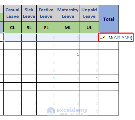
- Drag the Fill Handle icon down.
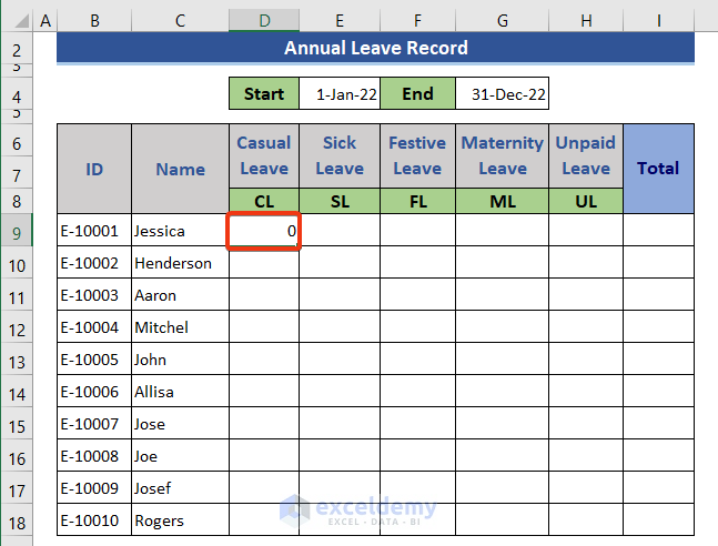
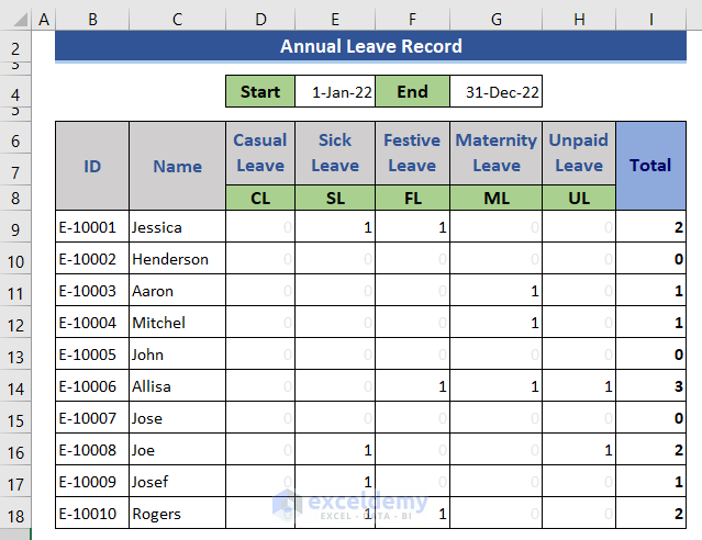
Step 5 – Calculate Annual Leaves
- Copy the last worksheet and customize a new worksheet for calculation.
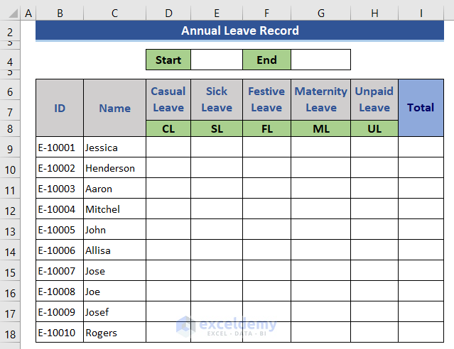
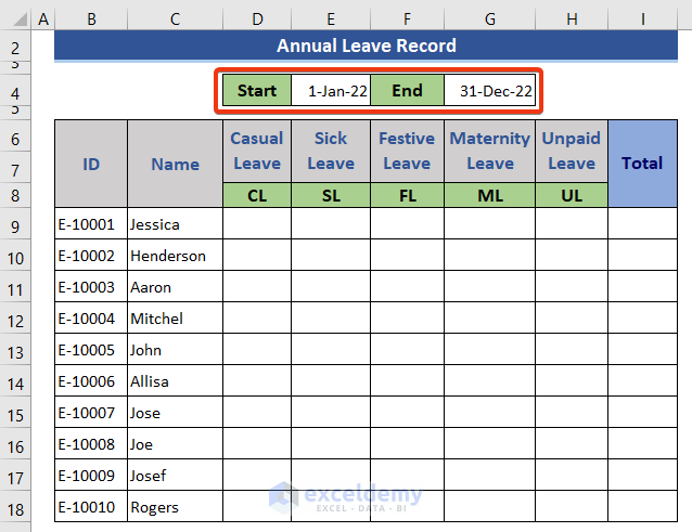
- We have two cells for Start and End. We input dates here. We start on 1st January and end on 31st December.
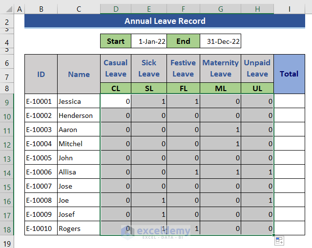
- Input this formula in D9.
=COUNTIFS(Record!$E:$E,">="&'Annual Leave'!$E$4,Record!$E:$E,"<="&'Annual Leave'!$G$4,Record!$C:$C,'Annual Leave'!$B9,Record!$F:$F,'Annual Leave'!D$8)
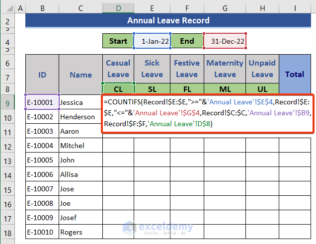
- Press the Enter button.
- Expand the formula to the whole leave area.
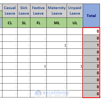
- Apply a SUM formula at cell I9 for total leaves.
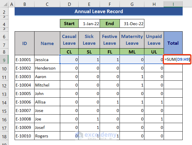
- Press the Enter button and drag the Fill Handle icon down.
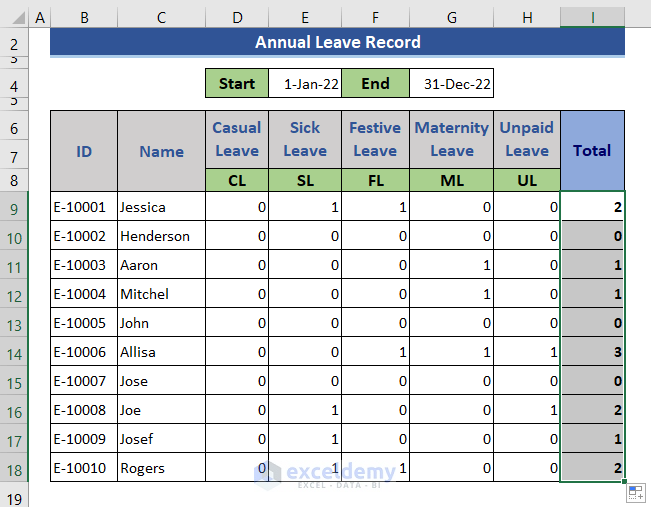
- Apply the conditional formatting to remove the 0 (zero) values.
Download the Template
<< Go Back to Leave Calculation | Formula List | Learn Excel
Get FREE Advanced Excel Exercises with Solutions!

Hi,
I try use below mentioned formula but why I cant add 2 lookup value..($B9&D$7)
=IFERROR(VLOOKUP($B9&D$7,Record!$B:$F,5,FALSE),””)
Hello KO,
Thank you very much for your comment. The formula you mentioned in the comment is working smoothly from our side. If you share your workbook, we will be able to find out the solution to your problem. You can mail us at [email protected].
Is there any formula for a drop down list using different type of leaves in the attendance sheet that data will not able to move if I jump in to different month.
Dear Prince,
Thank you very much for reading our article.
According to your query, 1st you wanted to know about a formula to create a drop-down list that will be used to select different types of leaves. You will get that in Step 3 of this article. In our Excel file, we selected leave using the drop-down list in Record sheet. Also when you move to any month leave information will be based on the Record sheet. So, information will not move from one month to another. Try this and hope you will get the solution.
Otherwise, send your Excel file with what you want to get and we will try to provide a solution. You can mail us at [email protected].
Thanks
Joyanta Mitra
ExcelDemy
On the third step where the leave record is captured. Is there way to make it so that instead of recording individual days of leave, it will rather be a range of say two days or five days.
Hello Chris
Thanks for your comment! You want to insert multiple leave records at a time.
I have reviewed your requirements. I am delighted to inform you that I have found an idea that uses an Excel UserForm to fulfil your goal. Please check the following:
To improve the Excel file, I had to write many lines of code and adjust many features, so I am not explaining how I did this. You can down the improved file from the following link: https://www.exceldemy.com/wp-content/uploads/2024/06/Chris-SOLVED.xlsm
Hopefully, you will like the idea. Good luck.
Regards
Lutfor Rahman Shimanto
Excel & VBA Developer
ExcelDemy
will this formula also work with leave donations and administrative leave?
Hello Doreen Bagola,
The formula we used to calculate annual leave can be adjusted for leave donations and administrative leave, but you’ll likely need to customize it depending on how these types of leaves are tracked.
For instance, you can add extra columns or rules to include donated or administrative leave alongside the regular annual leave calculations. This will ensure all leave types are accounted for. You may need to adjust data validation or leave balance formulas accordingly.
Regards
ExcelDemy
How can I make it where the spreadsheet shows hours instead of days?
Hello Satarrah,
Yes, you can show the annual leave balance in hours instead of days by converting the day-based result into hours.
For example, if your leave balance is calculated in days and one working day equals 8 hours, you can use:
=Leave_Days*8
So, if the remaining leave is in cell G2, use:
=G2*8
Then change the column header from Remaining Leave (Days) to Remaining Leave (Hours).
If your company uses a different daily working hour, such as 7.5 hours, use:
=G2*7.5
You can also modify the main leave calculation formula directly by multiplying the final result by the number of working hours per day.
Regards,
ExcelDemy