Step 1 – Create a Dataset and a Table
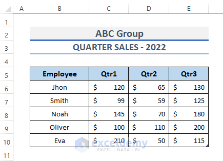
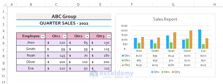
- We’ll use a sample dataset for a company’s quarterly sales in 2022. This contains employee names and the sales of quarters 1, 2, and 3.
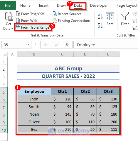
- Select the whole dataset. We selected the range of cell B5:E10.
- Go to the Data tab of the ribbon.
- Under Get & Transform Data, select From Table/Range.
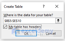
- This will display the Create Table dialog box.
- In the ‘Where is the data for your table?‘ box, you can see the range of the table.
- Check My table has headers.
- Click on the OK button to create the table.
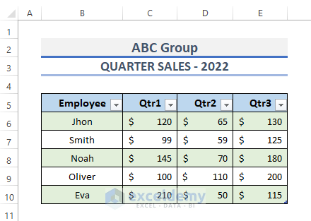
- The table has been created.
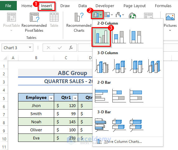
Step 2 – Insert a Chart
- Go to the Insert tab on the ribbon.
- In the Charts category, click on the Insert Column or Bar Chart drop-down menu.
- Select the first chart from the 2-D Column.
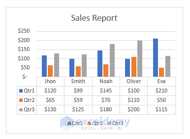
- Here’s the sample data chart.
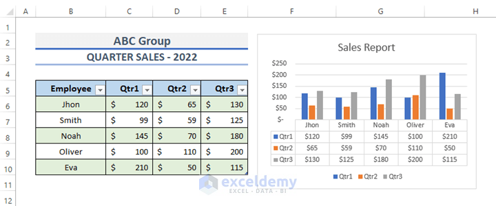
- The spreadsheet looks like this.
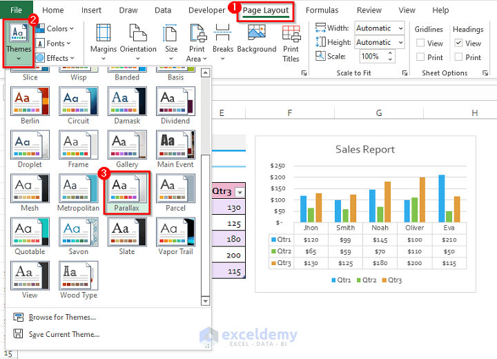
Step 3 – Apply the Theme from Page Layout
- Go to the Page Layout tab from the ribbon.
- Under the Themes group, click on the Themes drop-down menu.
- Scroll down and click on the Parallax theme.
Related Article: How to Apply Slice Theme in Excel
Final Output
This is the final result after applying the parallax theme.
Note: To change theme colors or for changing theme fonts:
- Select Colors, modify Colors or Fonts, and configure Fonts on the Page Layout tab’s Themes group.
- Under Themes, select Save Existing Style to save the chosen style to the File Themes directory.
- This template is now available for use in all of our worksheets. This template is also compatible with Word and PowerPoint.
Download the Practice Workbook
Related Articles
- How to Add Excel Feathered Theme
- [Solved!] Excel Themes Option Is Not Working
- [Solved!] Excel Feathered Theme Missing
- How to Change Excel Theme to Black
- How to Make Good Excel Color Combinations
- How to Create an Excel Theme
<< Go Back to Excel Theme | Learn Excel
Get FREE Advanced Excel Exercises with Solutions!
