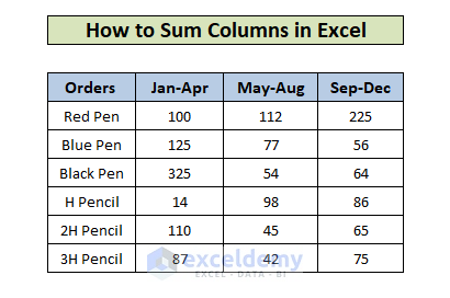
The following dataset represents the order summary of 6 products.
To show details of the orders throughout the year:
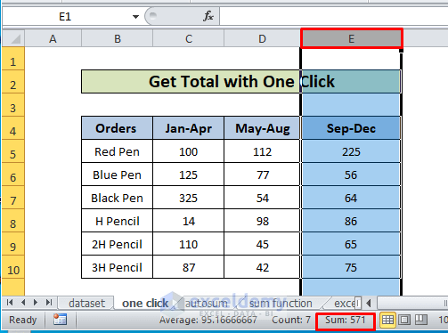
Method 1 – Getting the Sum of a Column in Excel with One Click
- Select a Whole Column: Click the letter of the column. The Excel status bar will show the sum along with the cells count.
- Selected Cells of a Column: select cells and the status bar will show the value of the summed data.
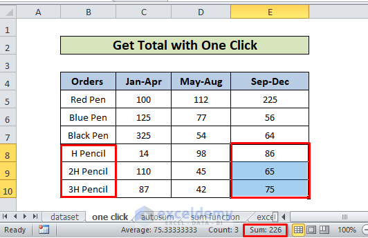
Here, E8:E11 was selected to get the total for pencils during Sep-Dec.
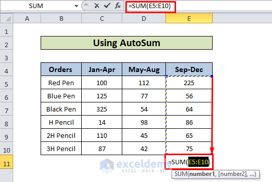
Method 2 – Using the AutoSum Command to Sum Columns in Excel
- Select the empty cell below the cells you want to add.
- In the Home tab, click AutoSum in Editing.
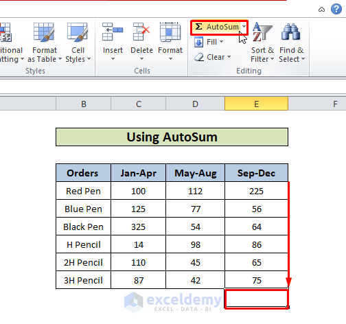
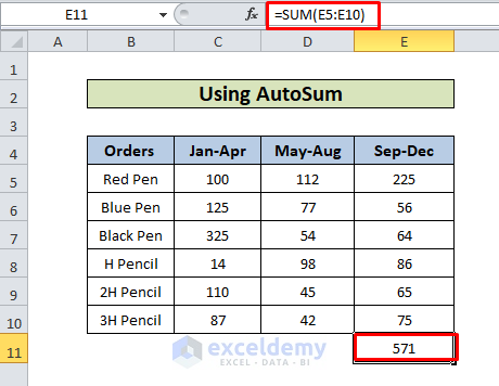
- Excel return the result of the SUM function.
- Press Enter key to see the column total in C11.
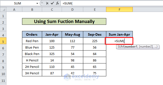
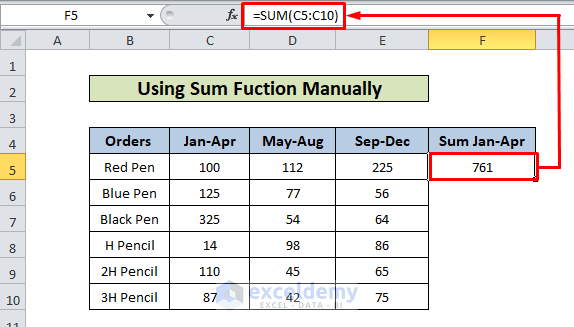
Method 3 – Calculating the Total by Entering the SUM Function Manually
- Select a cell to see the summed value and enter the SUM function.
- Select C5:C10.
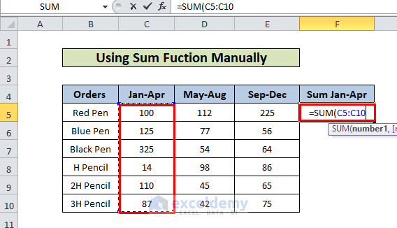
- Press Enter key to see the result.
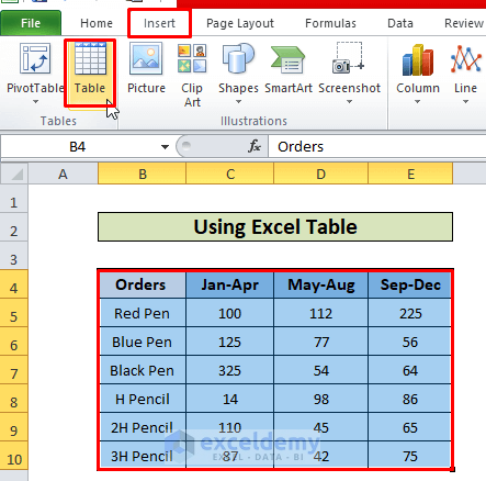
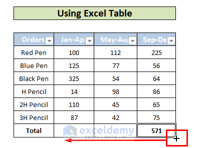
Method 4 – Transforming Data into an Excel Table to Sum Columns
- Select the dataset.
- In the Insert tab, choose Table.
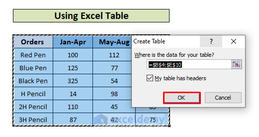
- Click OK in Create Table. This will turn the dataset into an Excel table.
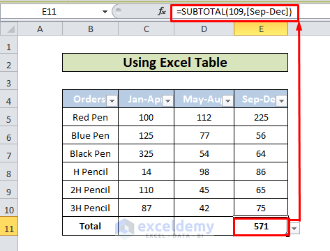
- Go to Design and check Total Row.

- The sum is displayed in E11.
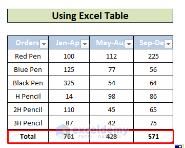
- To get the totals for the other columns (Jan-Apr and May-Aug), Drag the Fill Handle to the left.
- This is the output.
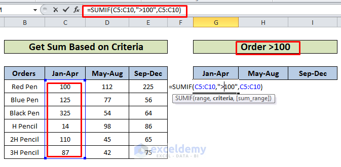
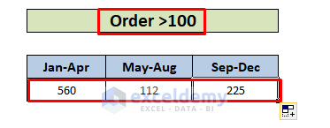
Method 5 – Adding a Column Based on Criteria
Sum orders greater than 100 in the three periods of time:
- Select a cell to see the summed value and enter the function.
=SUMIF(C5:C10,">100",C5:C10)- Press Enter.
- 560 is the sum of 125, 325, and 110.
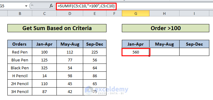
- Use the Fill Handle to see the result in the other cells.
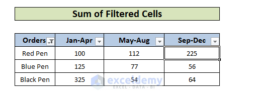
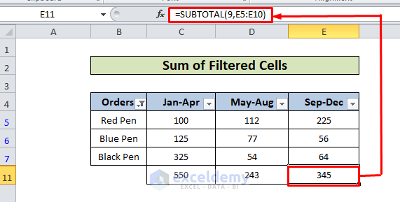
Method 6 – Calculating the Subtotal of Filtered Cells
To get the total of visible data only:
- Select the columns to filter.
- In the Data tab select Filter.
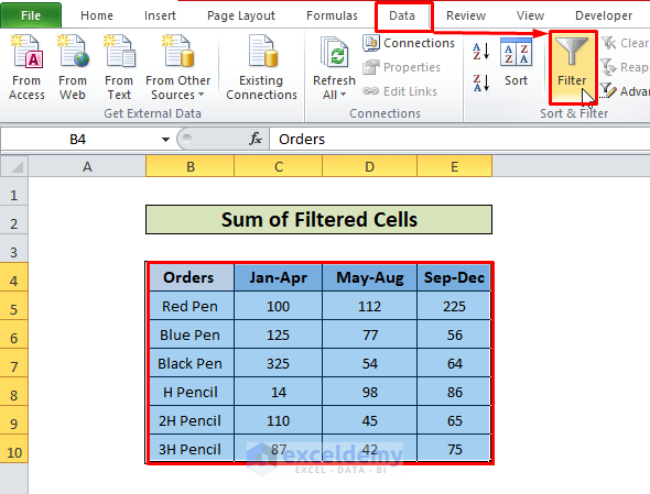
- A filter arrow will be displayed.
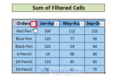
- Click the arrow and choose pens (Black, Red, and Blu).
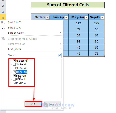
- The dataset is filtered.
- Use the AutoSum to calculate totals for the columns.
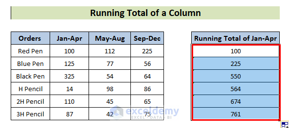
Method 7 – Finding the Running Total of an Excel Column
- In the first cell of the Running Column of Jan-Apr column, enter the following formula
=SUM(C$5:C5)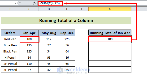
- Drag down the Fill Handle to the bottom of the column.
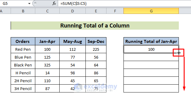
This is the output.
Download Practice Workbook
Download the practice workbook.
How to Sum Columns in Excel: Knowledge Hub
<< Go Back to How to Sum in Excel | How to Calculate in Excel | Learn Excel
Get FREE Advanced Excel Exercises with Solutions!
