How to Sum Columns in Excel When Filtered (7 Ways)

We use the filter function quite often because of its ability to churn up the most important insights of the data, which helps us immensely to make decisions using data. This article tries to answer how to sum columns in Excel when filtered most efficiently and simplistically.

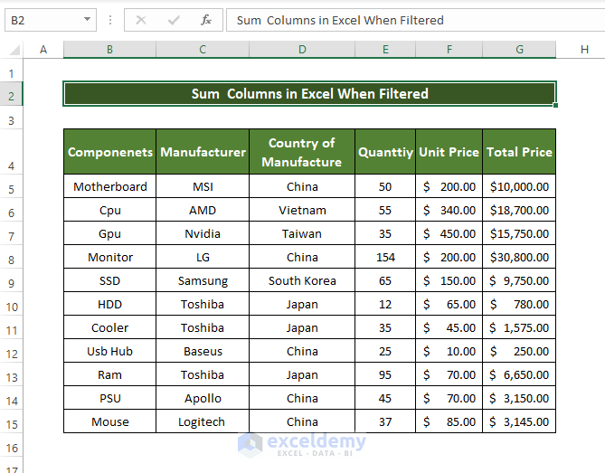
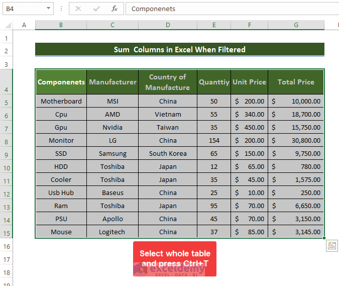
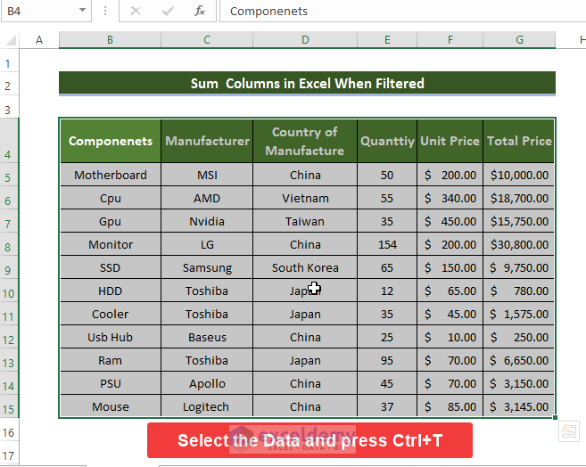
In this article, I am going to use this dataset for demonstrating purposes. We have Components, Manufacturer, Country of Manufacture, Quantity, Unit Price, and Total Price as the column header. We will try to filter these prices based on various criteria and those processes will be explained with broad demonstrations.

1. Using SUBTOTAL Function to Sum Columns in Excel When Filtered

The SUBTOTAL function is the most common way to calculate the sum of columns dynamically. It is done through Ribbons and formulas.

1.1 Inserting SUBTOTAL from AutoSum Option

In this method, the SUBTOTAL method will be applied through the AutoSum Option in the Editing group.

Steps

• First, you need to make a table and apply AutoSum to it. For this, go to Data > Filter.

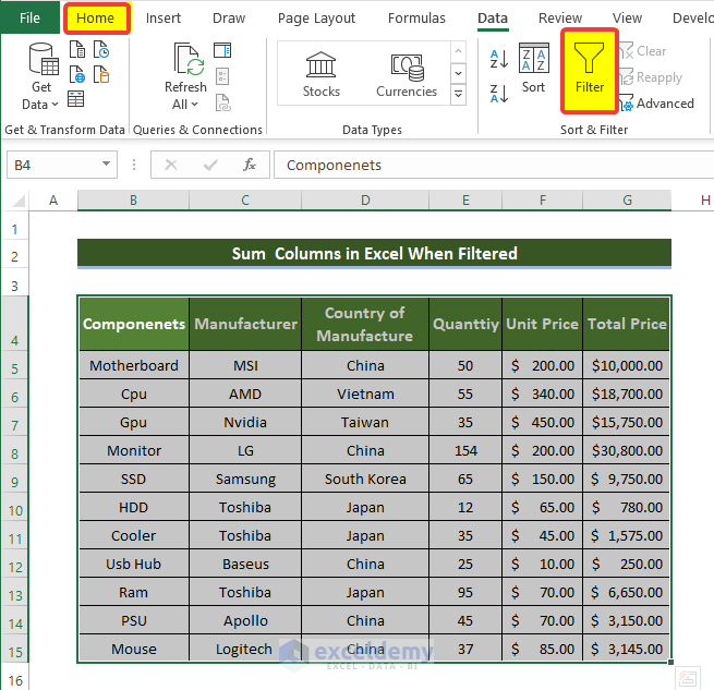
• After this, you will notice that the regular filter icon on every column header appears.

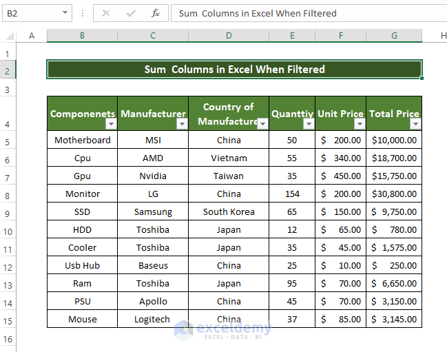
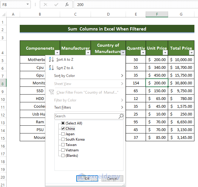
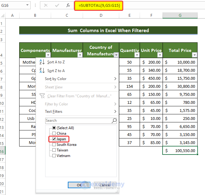
• Then we will try to filter the table by Country of Manufacture. To do this click on the arrow sign on the corner of the table header in cell D4.

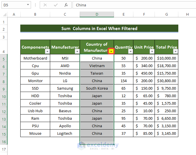
• After clicking the icon, check only the China option in the Text Filters option box, to show only the entries that belong to China. After that click OK.

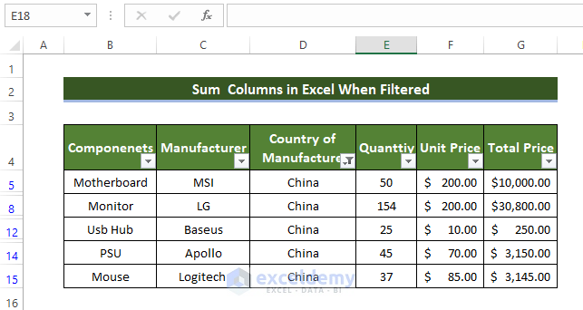
• Then you will notice that the table now shows only the entries that belong to China in the Country of Manufacture column.

• Next, select cell G17, and then from the Home tab go to Editing group and then click on the AutoSum option.

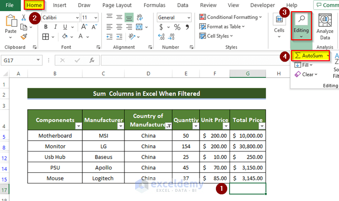
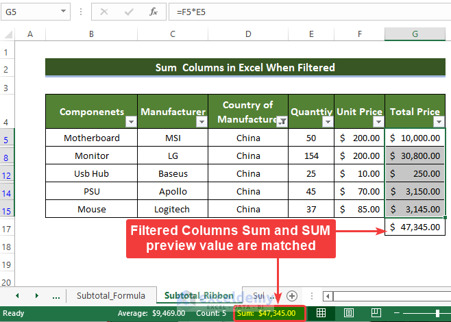
• After that you will see the SUBTOTAL function showing in cell G17, you need to select the data arrays in the Total Prize column and press Enter.

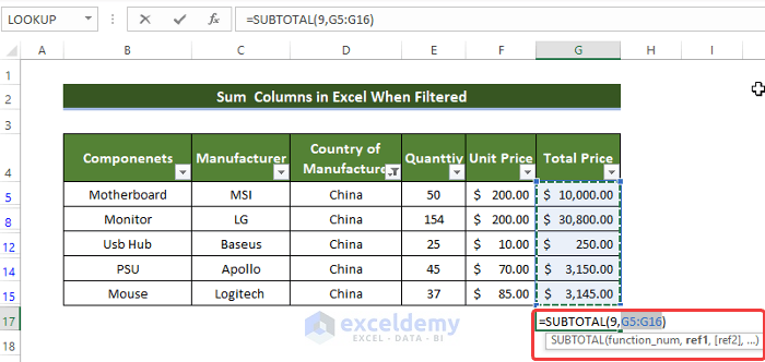
• After pressing enter you will notice your total summation of the filtered data is now showing properly. They also matched with the SUM preview below.

1.2 Applying Excel SUBTOTAL Function

Using the SUBTOTAL function, we can easily calculate the sum of column values after filtering is done.

Steps

• First of all, select the whole data set and press Ctrl+T. It will turn the selected dataset into an Excel table.

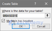
• After that, a new window will be created, and inside that table, you need to select the range of your dataset. Make sure to tick the My table has headers. Click OK after this.

• After clicking OK, you will observe that your data set is now converted into a table.
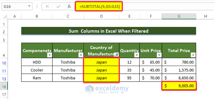
• Next, enter the following formula into the cell G16:

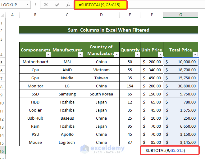
• After entering the formula, you will notice that the value of summation from the range of cells G5:G15 is now showing in cell G16.
• You can now filter the Country of Manufacture by clicking the corner box on cell D4.
• Then select Japan by checking the box and then click OK.

• After clicking OK, you will notice that your summation value at cell G16 is now updated for filtered value.

Read More: How to Sum Entire Column in Excel 

2. Calculating Total with Excel Table to Sum Filtered Columns

Utilizing the table row property of Excel tables you can calculate the sum of filtered cells quite easily.

Steps

• First of all, select the whole data set and press ‘Ctrl+T’. It will turn the selected dataset into an Excel table.

• After that, a new window will be created, and inside that table, you need to select the range of your dataset. Make sure to tick the My table has headers. Click OK after this.

• After clicking OK, you will observe that your dataset is now converted into a table.
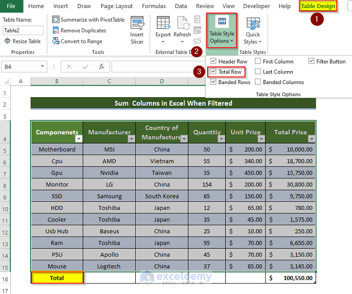
• Now go to Table Design > Table Style Options. Then check the Total Row box.
• Next, you will observe a row below the existing dataset created, Total in cell B16, and a new dropdown menu at cell G16. From the dropdown menu select SUM and then you will see the total sum of the Total Price column.

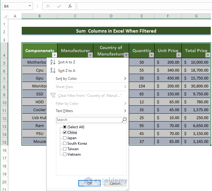
• Now if you select the drop-down sign in the corner of the Country of Manufacture cell and choose China, click OK.

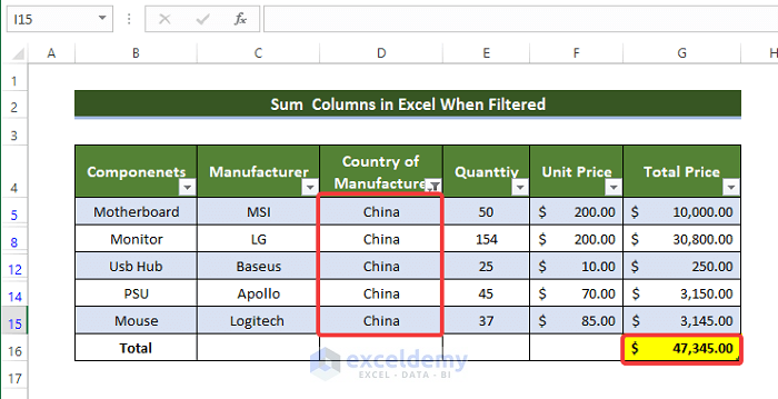
After clicking OK, you will notice that only China entries are filtered in, and the summation value is now updated for filtered entries.

3. Inserting AGGREGATE Function to Sum Columns

The AGGREGATE function can get the sum value of columns after they are filtered out.

Steps

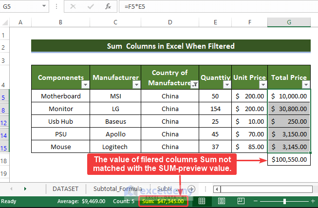
• To understand why AGGREGATE functions are needed, we first demonstrate why SUM functions don’t work in traditional worksheets.
• First, make a table from you dataset that you created before, and from that filter choose entries from only Japan or the country of Manufacture columns.
• Then enter the SUM function and select the Total Price column as an array argument.

• Then you will notice that the summation we got is not actually the summation of filtered cells, instead, it takes all the cell values from the range of cells G5:G15. Which is 11 value instead of the filtered 4 value. It is evident that the value from the SUM preview and summation of selected cells doesn’t match.

To counter this issue, using the AGGREGATE function could be helpful.

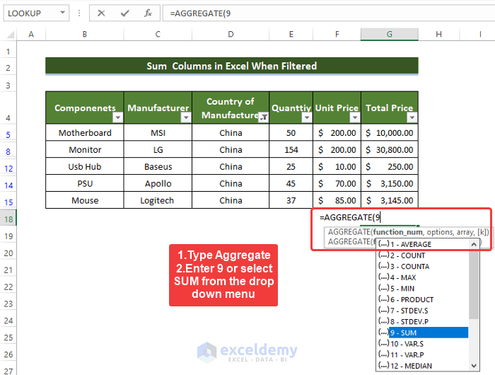
• To implement this, first enter the AGGREGATE  function in cell G16 after filtering out the desirable value, in this case, China filtered out.
• The first argument should be 9 or select SUM from the drop-down menu.

• Then type 5 or select Ignore hidden rows values from the drop-down menu.

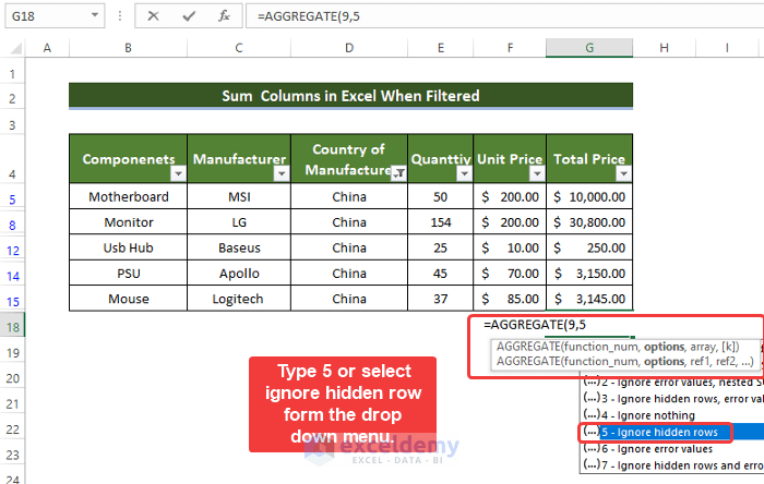
• Finally, select the array of cells whose summation you need to get.

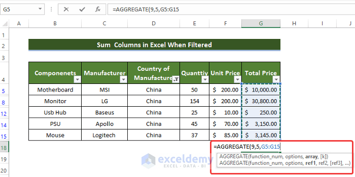
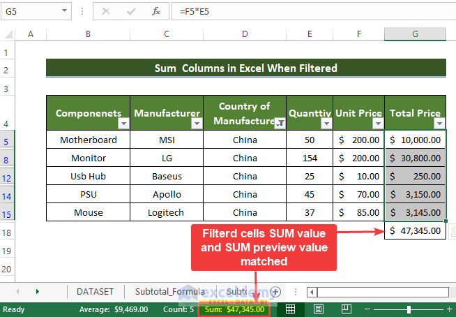
• After that, you can see that the filtered cells’ SUM value matches perfectly with the SUM preview value shown below. This further confirms that this summation accurately calculates only entries from China.

Read More: How to Sum Columns by Color in Excel 

4. Applying VBA Macro to Sum Columns When Filtered

Using a simple VBA Macro can drastically reduce the time to Extract part of text from a long string.

Steps

• First, go to the Developer tab, then click Visual Basic.

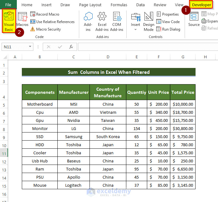
• Then click Insert > Module.

• In the module window, enter the following code:

Function SumColumn(Wr As range) As Double
Dim y As range
Dim x As Double
For Each y In Wr
If y.Rows.Hidden = False And y.Columns.Hidden = False Then
x = x + y.Value
End If
Next
SumColumn = x
End Function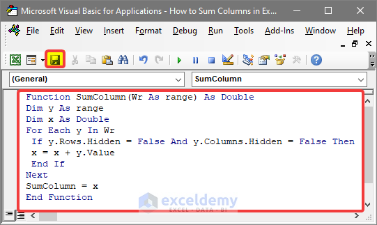

• Then close the window.
• After that select the whole window and press Ctrl+T.

• A new small window will open asking for the range of the table, select the range and check that My table has headers box.

• Now the whole dataset is converted to a table, enter the new formula just created through VBA in cell G16 :

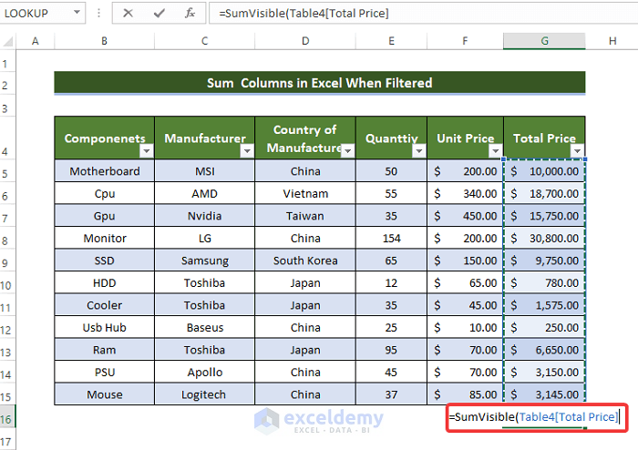
• After entering the data you will see the total value of prices listed in cell G16.
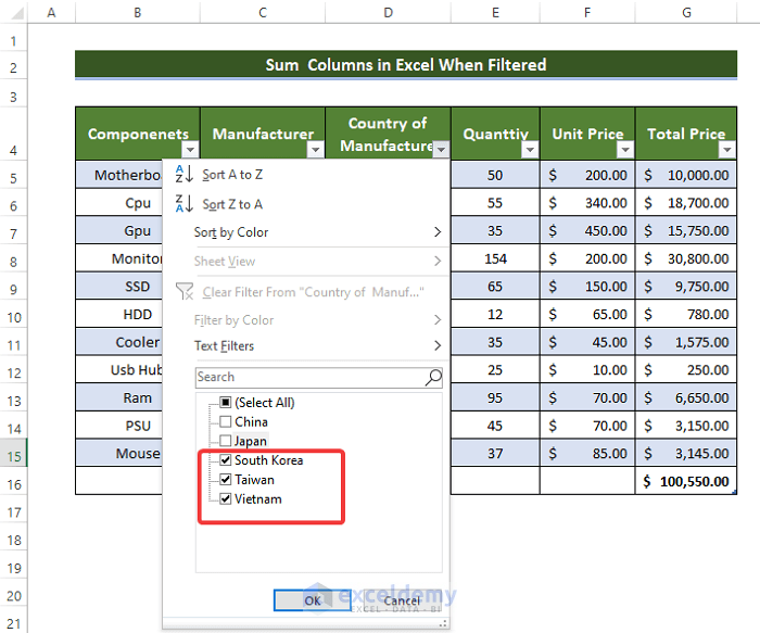
• Now, click the filter arrow icon on the corner of the County of Manufacturing column and choose South Korea, Taiwan, and Vietnam. Click OK after that.

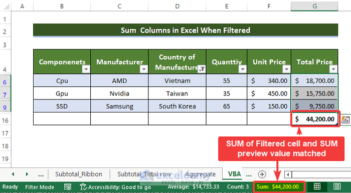
• After that, you will see the updated sum with only the filtered cells shown which matched exactly with the SUM preview value.

So, we can say, our method worked successfully to sum columns in Excel when filtered.

Read More: How to Sum Every Nth Column in Excel

Download Practice Workbook

Download this practice workbook below.

Conclusion

To sum it up, the question “How to Sum ColumnS in Excel when filtered” is answered here in 3 different ways. Among them, the SUBTOTAL method is actually into 3 sub-methods and explained accordingly, continuing to use the AGGREGATE function, ended up using VBA Macros. Among all of the methods used here, using the SUBTOTAL ribbon method is the easier-to-understand-and simpler one. The VBA process is also less time-consuming and simplistic but requires prior VBA-related knowledge. Other methods don’t have such a requirement.
For this problem, a macro-enable workbook is available for download where you can practice these methods.

Related Articles

• How to Calculate Total Row and Column in Excel
• How to Sum Multiple Rows and Columns in Excel
• How to Total a Column in Excel 
• How to Sum Columns in Excel Table

<< Go Back to Sum Columns | Sum in Excel | Calculate in Excel | Learn Excel