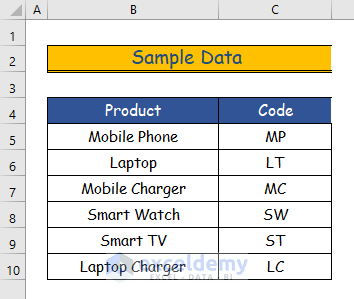
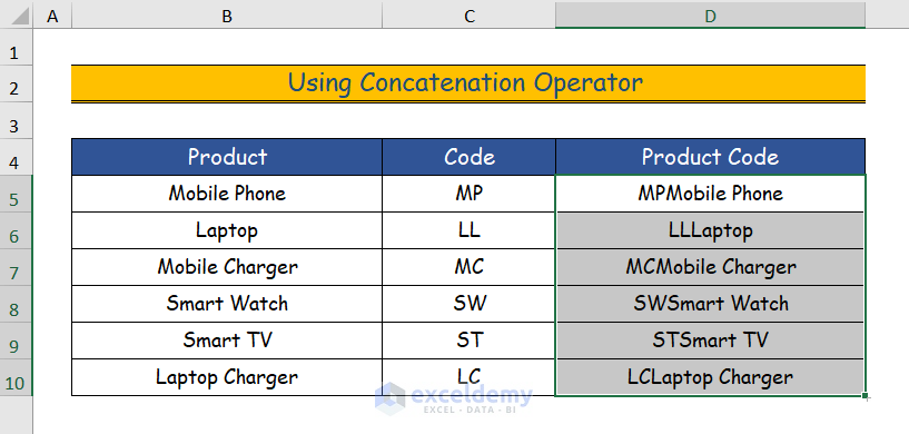
This is the sample dataset.
Method 1- Using the Ampersand Operator to Add Text in Excel
1.1 Using the Ampersand Operator to Add Text Without a Space
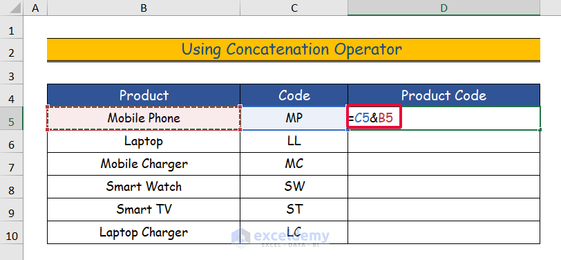
Step 1:
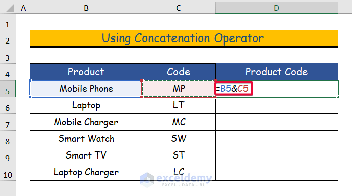
- Select the cell to add the text. Here, D5.
- Enter the formula below
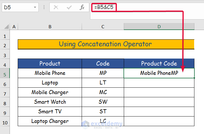
=B5&C5
- Enter the equal sign(“=”) in that cell.
- Choose the text you want to add. Here, text in B5 cell.
- Enter the concatenation operator (“&”).
- Select the next text you want to add. Here, C5.
- Press Enter.
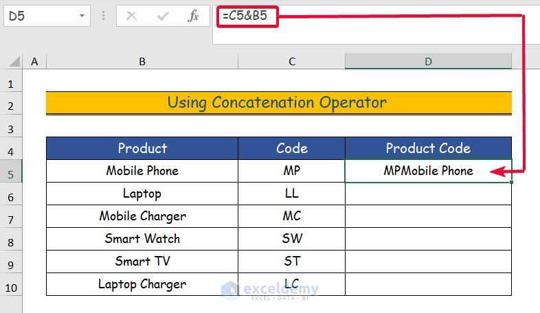
Step 2:
This is the output.
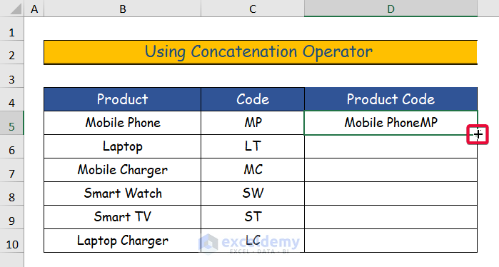
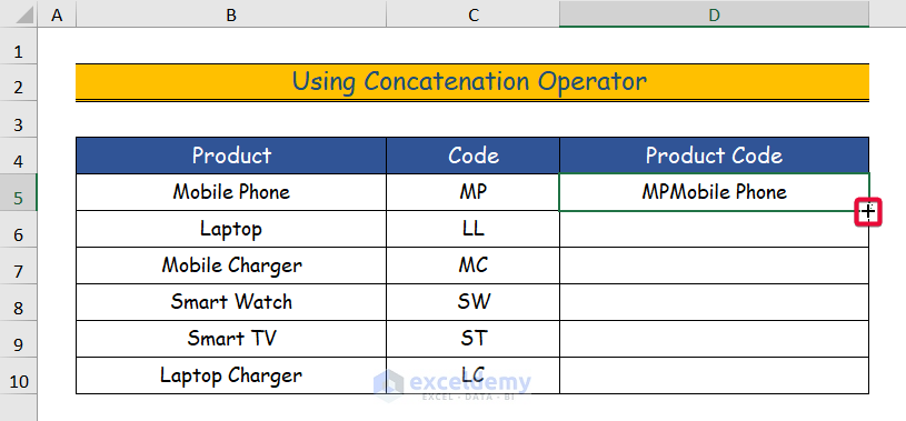
Step 3:
- Hover down to the bottom right corner of the cell containing the added text.
- A small plus sign will be displayed.
Step 4:
- Drag the cursor down.
- The rest of the cells will be auto-filled with the added text.
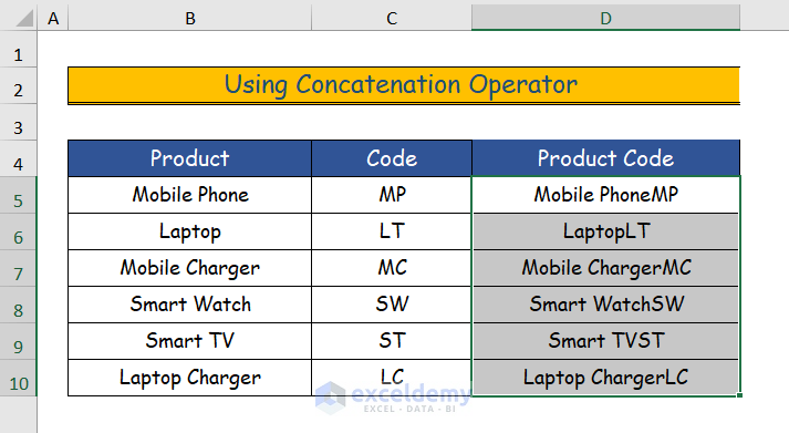
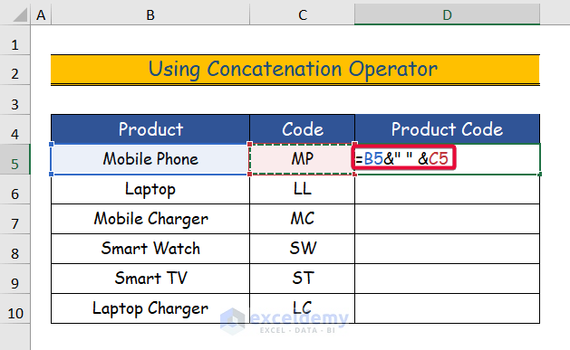
1.2 Utilizing the Ampersand Operator to Add Text with Space
Step 1:
- Select the cell to add the text. Here, D5.
- Enter the formula below
=B5&” “&C5
- Enter the equal sign (“=”).
- Select the text. Here, text in B5.
- Enter the concatenation operator (“&”) after it.
- Enter ” “. This means a space.
- Choose the text to add. Here, in C5.
- Press Enter.
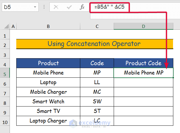
Step 2:
This is the output.
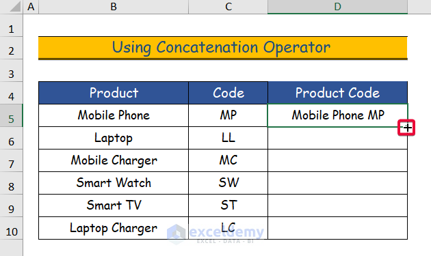
Step 3:
- Click the plus sign.
Step 4:
- Drag it down to the dataset’s final cell.
This is the output.
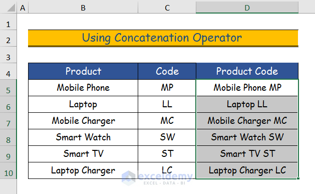
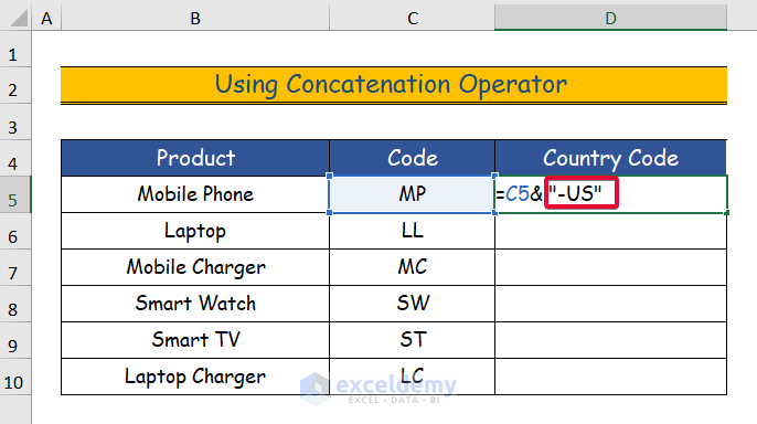
1.3 Using the Ampersand Operator to Add Text at the End of a String
Step 1:
- Select the cell to add the text. Here, D5.
- Enter the formula below.
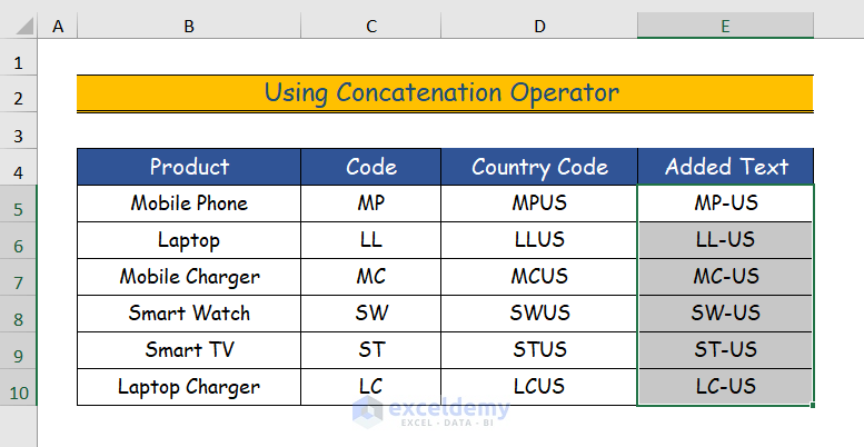
=C5&”-US”- Enter the equal sign (“=”) in that cell.
- Choose the first text. Here, in B5.
- Enter the “&” sign.
- Enter the text that you want to add at the end of the previous string.
- Here “-US”.
- Press Enter.
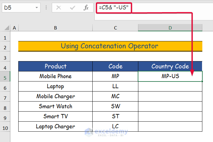
Step 2:
This is the output.
Step 3:
- Select the plus sign.
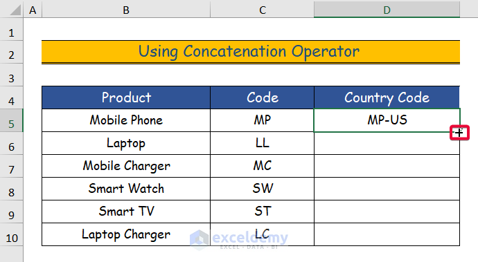
Step 4:
- Drag it down to the last cell of the dataset.
This is the output.
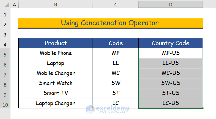
1.4 Applying the Ampersand Operator to Add Text After Nth Character
Step 1:
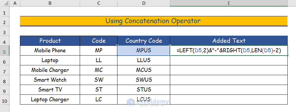
- Select the cell to add the text. Here, E5.
- Enter this formula.
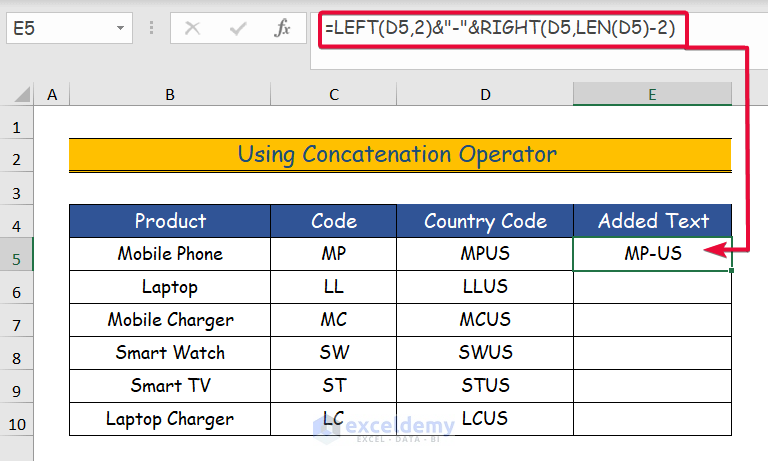
=LEFT(D5,2)&"-"&RIGHT(D5,LEN(D5)-2)- Press Enter.
Formula Breakdown
- LEFT(D5,2): The Left function extracts a substring from the left side of a text. It has two arguments: text and num_char. The text argument asks for the text from which the function will extract a substring, and the num_char argument asks for the number of characters the substring contains. It will return “MP”.
- RIGHT(D5,LEN(D5)-2): The RIGHT function works like the LEFT function except for the fact that it extracts a substring from the right of a text. The LEN function measures the length of text. The LEN(D5) returns 4. The RIGHT function took the same arguments as the LEFT function. The RIGHT function extracts the rest of the string. The num_char argument of the RIGHT function is LEN(D5)-2 or 4-2 which equals 2. The RIGHT function returns the 2 characters from the right of the text. Here “US”.
- LEFT(D5,2)&”-“&RIGHT(D5, LEN(D5)-2): The ampersand sign or the concatenation operator adds the texts together. The texts will be the result of the LEFT function, “MP”, a dash sign “-” and the result of the RIGHT function, “US”.
Step 2:
- The “-” sign is added between the strings.
Step 3:
- Drag down the plus sign.
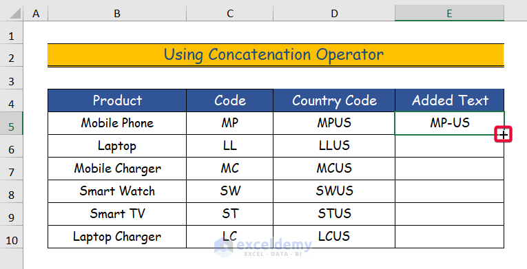
Step 4:
This is the output.
1.5 Using the Ampersand Operator to Combine Text from Two or More Cells
Step 1:
- Choose the cell to add text. Here, D5.
- Enter the formula below.
=C5&B5- Enter the equal sign (“=”) .
- Select the first text to add. Here, C5.
- Enter “&”.
- Select the text you want to add after the first one. Here, in B5.
- Press Enter.
Step 2:
The cell will display the concatenated text.
Step 3:
- Click the plus sign.
Step 4:
- Drag it down to the last cell of the dataset.
This is the output.
Read More: Add Text and Formula in the Same Cell in Excel
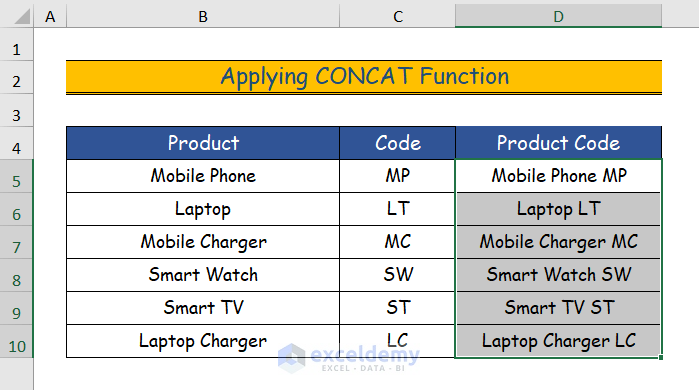
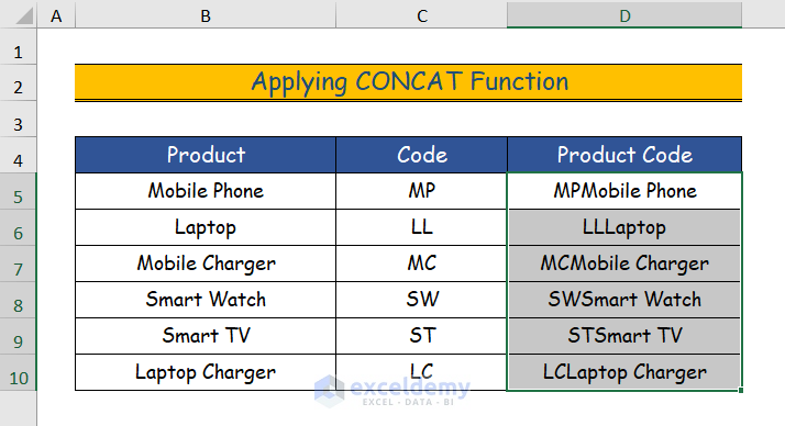
Method 2 – Applying the CONCAT Function to Add Text in Excel
2.1 Add Text Without Spaces
Step 1:
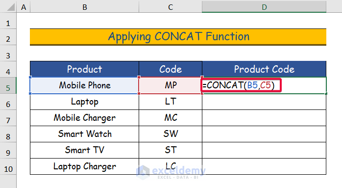
- Choose the cell to add the text. Here, D5.
- Use the following formula with the CONCAT function.
=CONCAT(B5,C5)- Enter the equal sign (“=”).
- Enter “CONCAT”, and the CONCAT function will appear.
- Select the first text. Here, B5.
- Enter a comma.
- Select the text you want to add by clicking it. Here, C5.
- Press Enter.
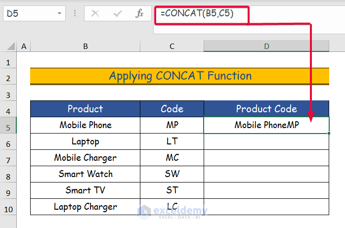
Step 2:
The cell will display the concatenated text.
Step 3:
- Click the plus sign.
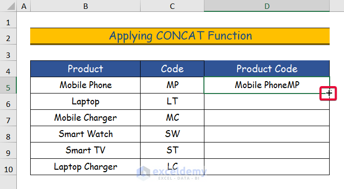
Step 4:
- Drag it down to the final cell.
This is the output.
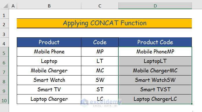
2.2 Add Text with Space
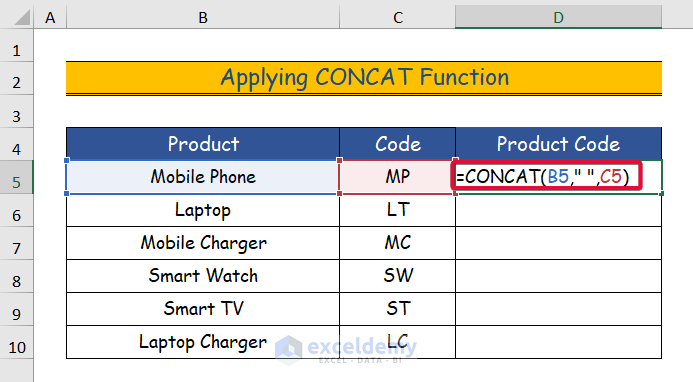
Step 1:
- Select the cell to add the text. Here, D5.
- Use this formula.
=CONCAT(B5,” “,C5)
- Enter the equal sign (“=”).
- Enter “CONCAT”, and the CONCAT function will appear.
- Select the first text. Here, B5.
- Enter a comma.
- Add a double quotation(“ “) with a space.
- Select the text you want to add. Here, in C5.
- Press Enter.
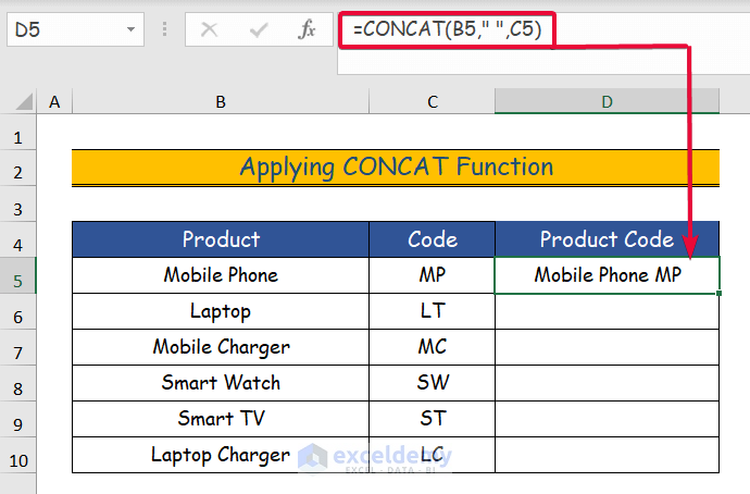
Step 2:
The concatenated text will be displayed.
Step 3:
- Click the plus sign.
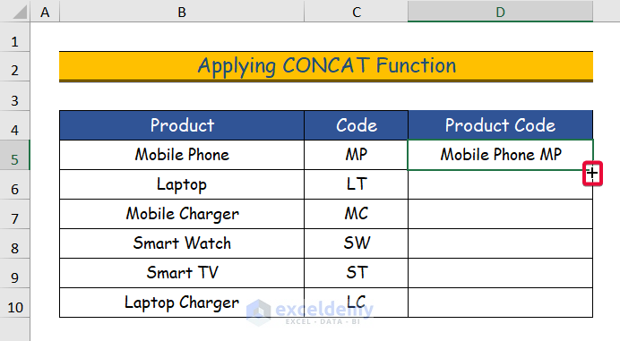
Step 4:
- Drag it down to the final cell.
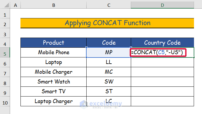
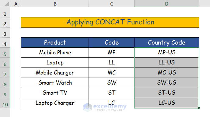
2.3 Add Text at the End of a String
Step 1:
- Select the cell to add the text. Here, D5.
- Use this formula.
=CONCAT(C5,”-US”)
- Enter the equal sign (“=”).
- Enter “CONCAT”, and the CONCAT function will appear.
- Select the first text. Here, B5.
- Enter a comma.
- Add a double quotation(“ “) with a space.
- Enter the text you want to add. Here “-US”.
- Press Enter.
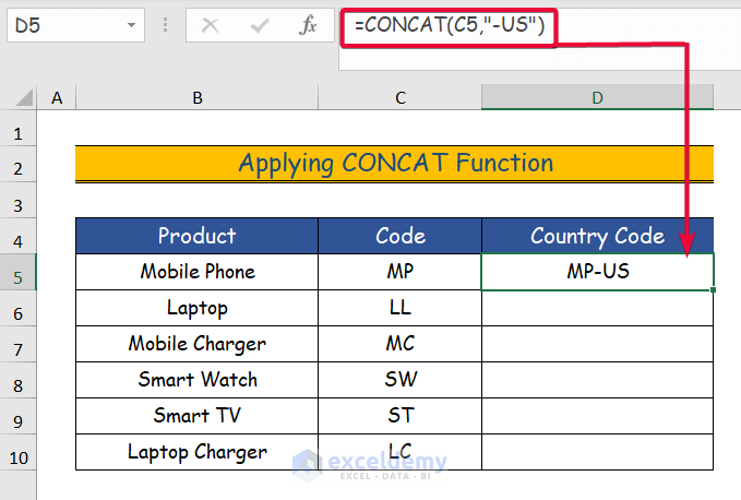
Step 2:
The text will be added at the end of the string.
Step 3:
- Click the plus sign.
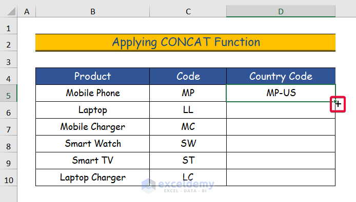
Step 4:
- Drag it down to the final cell.
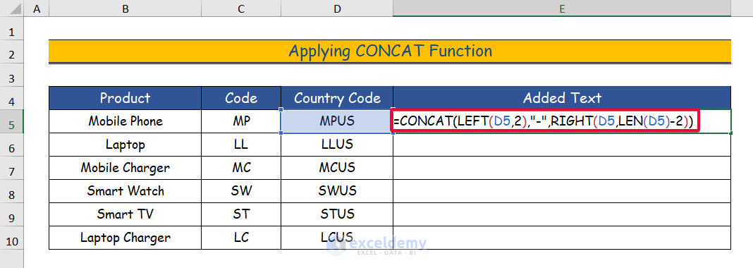
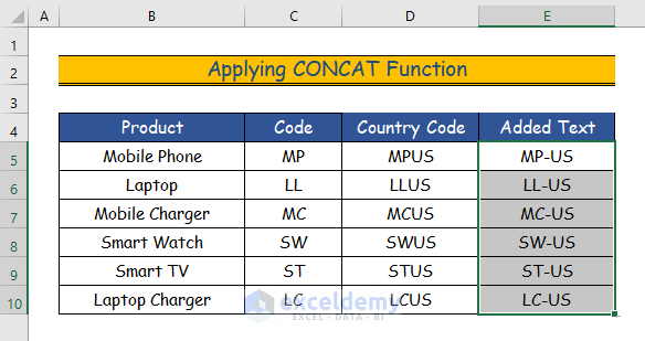
2.4 Add Text After Nth Character
Step 1:
- Select the cell to add the text. Here, E5.
- Use this formula.
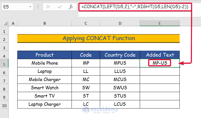
=CONCAT(LEFT(D5,2),"-",RIGHT(D5,LEN(D5)-2))- Press Enter.
Formula Breakdown
- LEFT(D5,2): The Left function extracts a substring from the left side of a text. It has two arguments: text and num_char. The text argument asks for the text from which the function will extract a substring, and the num_char argument asks for the number of characters the substring will contain. It will return “MP”.
- RIGHT(D5,LEN(D5)-2): The RIGHT function works like the LEFT function except for the fact that it extracts a substring from the right of a text. The LEN function measures the length of text. It returns 4. The RIGHT function takes the same arguments as the LEFT function. The RIGHT function extracts the rest of the string left by the LEFT function. The num_char argument of the RIGHT function is LEN(D5)-2 or 4-2 which equals 2. The RIGHT function returns the 2 characters from the right of the text. Here, “US”.
- CONCAT(LEFT(D5,2),”-“,RIGHT(D5,LEN(D5)-2)): The CONCAT function adds the texts. The texts will be the result of the LEFT function, “MP”, a dash sign “-” and the result of the RIGHT function, “US”.
Step 2:
- A “-“ symbol is added.
Step 3:
- Click the plus sign.
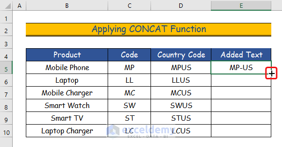
Step 4:
- Drag it down to the final cell.
Read More: How to Add a Word in All Rows in Excel
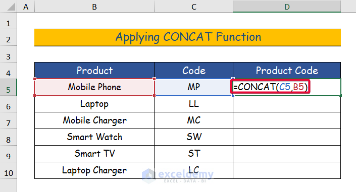
2.5 Combine Text from Two or More Cells
Step 1:
- Select the cell to add the text. Here, D5.
- Use this formula.
=CONCAT(C5,B5)- Enter the equal sign (“=”).
- Enter “CONCAT”, and the CONCAT function will appear.
- Select the text to add. Here, C5.
- Enter a comma.
- Select the text you want to add after the first one. Here, B5.
- Press Enter.
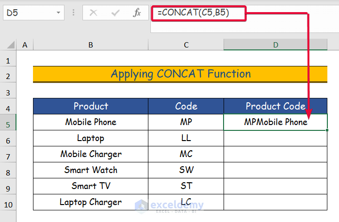
Step 2:
The combined text will be displayed.
Step 3:
- Click the plus sign.
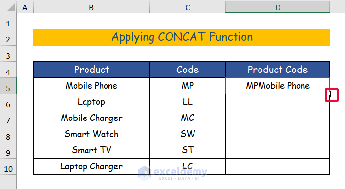
Step 4:
- Drag it down to the final cell.
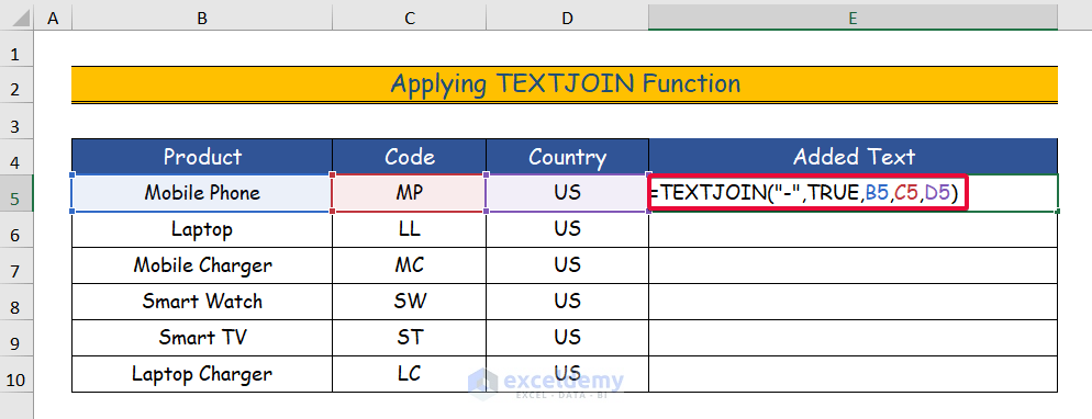
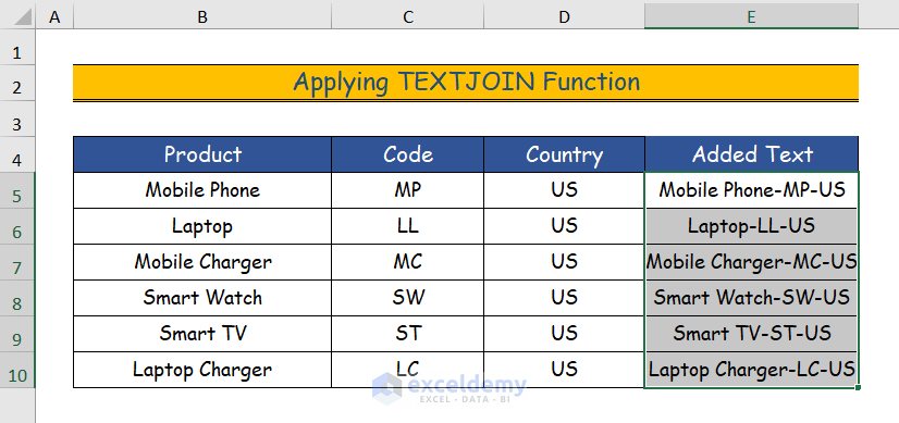
Method 3 – Applying the TEXTJOIN Function to Add Text in Excel
Step 1:
- Select the cell to add the text. Here, D5.
- Use this formula.
=TEXTJOIN(“-”,TRUE,B5,C5,D5)- Enter the equal sign followed by ”TEXTJOIN”. The TEXTJOIN function will appear.
- The first argument requires is a delimiter to separate the texts. Here, the dash sign.
- The next argument asks if it will ignore empty text. Choose TRUE .
- Choose the cells that you want to add separated by commas. Here, B5, C5, and D5 cells.
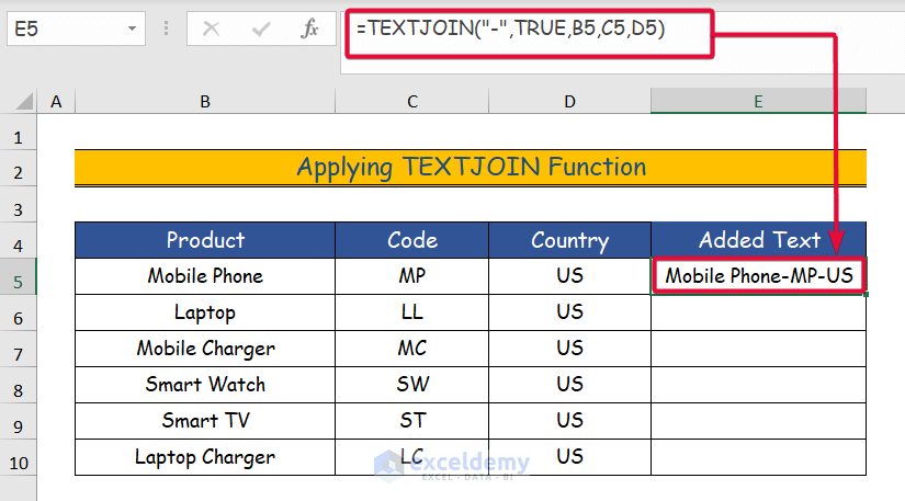
Step 2:
The combined text will be displayed, separated by a dash.
Step 3:
- Click the plus sign.
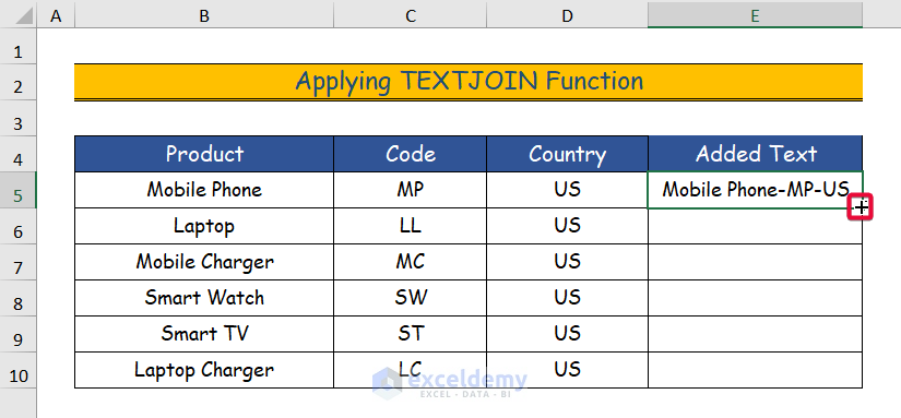
Step 4:
- Drag it down to the final cell.
Read More: How to Add Text to Multiple Cells in Excel
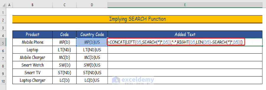
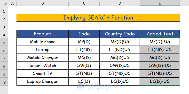
Method 4 – Using the SEARCH Function to Add Text in Excel
Step 1:
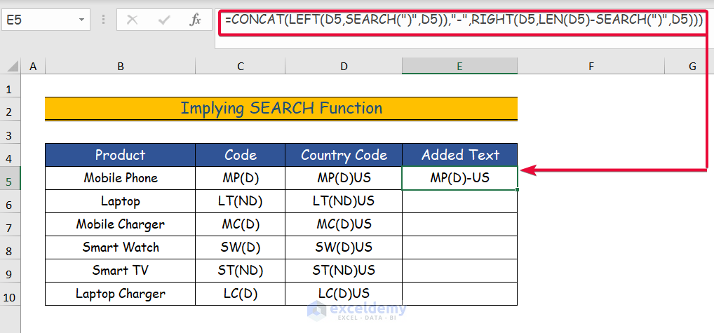
- Select the cell to add the text. Here, E5.
- Use this formula.
=CONCAT(LEFT(D5,SEARCH(")",D5)),"-",RIGHT(D5,LEN(D5)-SEARCH(")",D5)))- Press Enter.
Step 2:
- Between the strings, a “-“ symbol is added.
Formula Breakdown
- SEARCH(“)”,D5): The SEARCH function takes two arguments :find_text and within_text. The find_text argument asks for the text or the character to be searched. The within_text argument takes the text. Here, the SEARCH function will search for the “)” character in the text MP(D)US. The function returns the position of the character within the text in numeric value: 5.
- LEFT(D5,SEARCH(“)”,D5)): The Left function extracts a substring from the left side of a text. It has two arguments: text and num_char. The text argument asks for the text from which the function will extract a substring, and the num_char argument asks for the number of characters the substring contains. It returns “MP(D)”.
- RIGHT(D5,LEN(D5)-SEARCH(“)”,D5)): The RIGHT function works like the LEFT function except for the fact that it extracts a substring from the right of a text. The LEN function measures the length of text. The LEN(D5) returns 7. The RIGHT function takes the same arguments as the LEFT function. The RIGHT function extracts the rest of the string left by the LEFT function. The num_char argument of the RIGHT function is LEN(D5)-SEARCH(“)“,D5) or 7-5 which equals 2. The RIGHT function returns the 2 characters: “US”.
- CONCAT(LEFT(D5,SEARCH(“)”,D5)),”-“,RIGHT(D5,LEN(D5)-SEARCH(“)”,D5))): The CONCAT function adds the texts. The texts will be the result of the LEFT function,“MP(D)”, a dash sign “-” and the result of the RIGHT function, “US”.
Step 3:
- Click the plus sign.
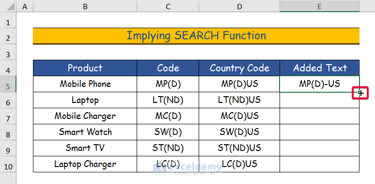
Step 4:
- Drag it down to the final cell.
Read More: How to Add Text to Cell Without Deleting in Excel
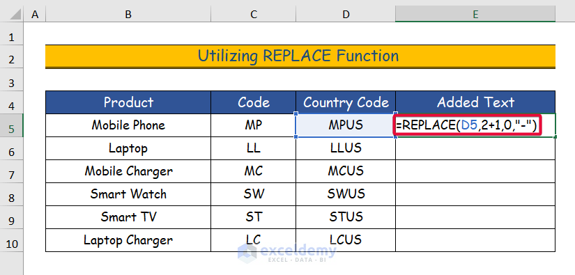
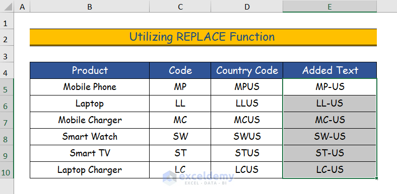
Method 5 – Utilizing the REPLACE Function
Step 1:
- Select the cell to add the text. Here, D5.
- Use this formula.
=REPLACE(D5,2+1,0,”-”)
- Enter “REPLACE” after the equal sign.
- The first argument is the text from which you want to replace a character with. Here, D5
- The next argument asks the position to replace the text. Here, 2+1 or the 3rd position.
- Enter 0. The formula adds text to the cell in the selected location without replacing.
- Choose the character you want to insert in that position. Here, “-”.
- Press Enter.
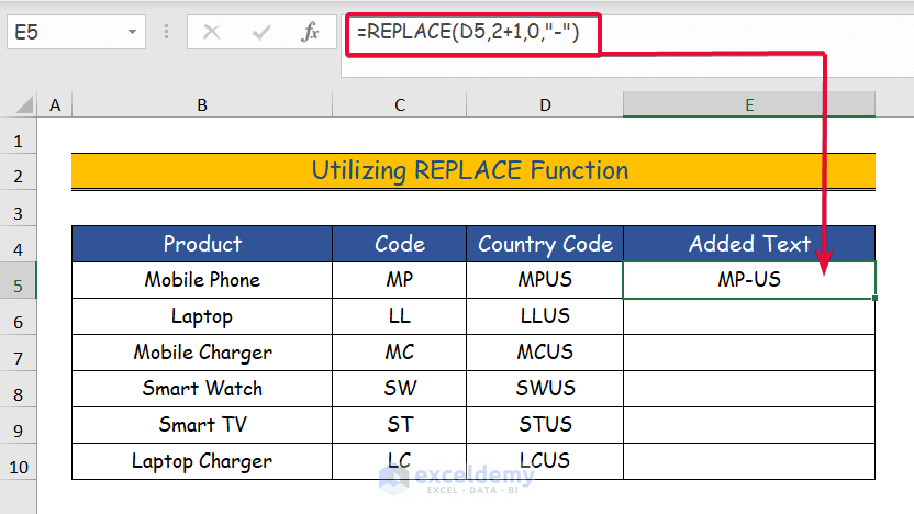
Step 2:
- The dash sign is added between the texts.
Step 3:
- Click the plus sign.
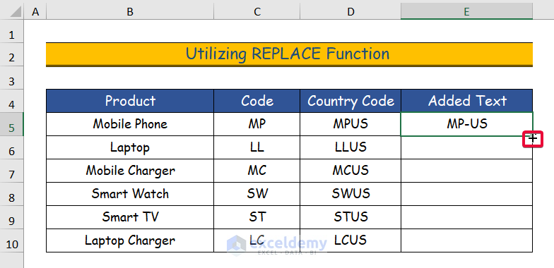
Step 4:
- Drag it down to the final cell.
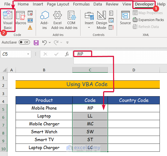
Method 6 – Using a VBA Code to Add Text
6.1 Add Text at the Beginning of a String
Step 1:
- Select the cells to which you will add a prefix. Here, C5:C10.

Step 2:
- Go to the Developer.
- Select Visual Basic.
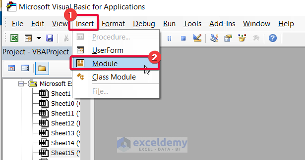
Step 3:
- Select Insert.
- Choose Module.
Step 4:
- Enter the code in the module.
Sub TextAtTheBeginning()
'declaring variables'
    Dim cellValues As Range
'running the for loop'
    For Each cellValues In Application.Selection
    'if statement implied'
        If cellValues.Value <> "" Then cellValues.Offset(0, 1).Value = "US-" & cellValues.Value
    Next
End Sub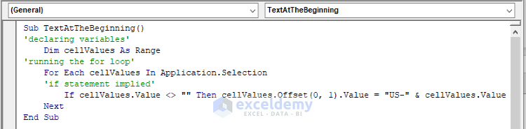
VBA Code Breakdown
- The function name is TextAtTheBeginning.
- The variable name is cellValues and it is a range type variable.
- For Each cellValues In Application.Slection: will run a for loop through each selected cell.
- If cellValues.Values<> “ “: If the values in the selected cells are not equal to zero.
- Then cellValues.Offset(0,1).Value= cellValues.Value & “-US”: The code will copy the cell value in the adjacent cell and add “-US” at the beginning.
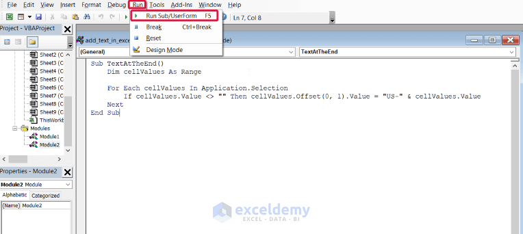
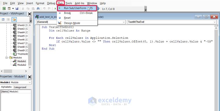
Step 5:
- Run the code.
Step 6:
The prefix “US-” is added.
Read More: How to Add Text in the Middle of a Cell in Excel
6.2 Add Text at the End of a String
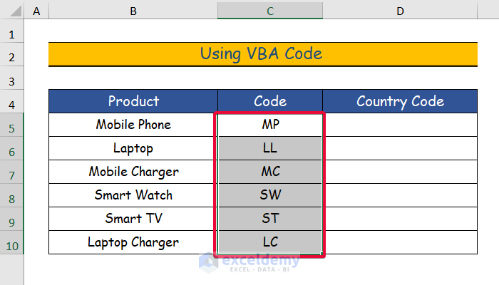
Step 1:
- Choose the texts in front of which you will add the suffix. Here, C5:C10.
Step 2:
- Select the Developer tab.
- Choose Visual Basic.

Step 3:
- Select Insert.
- Choose Module.

Step 4:
- Enter the code in the module.
Sub TextAtTheEnd()
'declaring variable'
   Dim cellValues As Range
 'running the for loop'
    For Each cellValues In Application.Selection
    'if statement implied'
        If cellValues.Value <> "" Then cellValues.Offset(0, 1).Value = cellValues.Value & "-US"
    Next
End Sub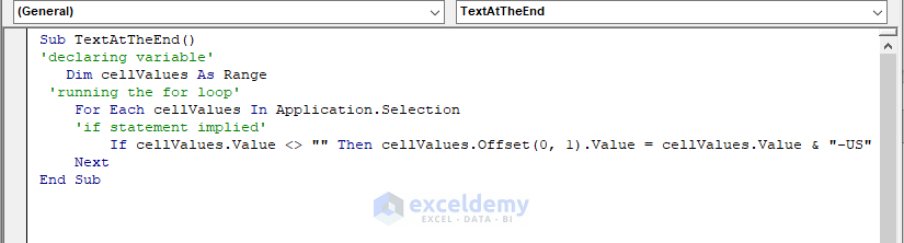
VBA Code Breakdown
- The function name is TextAtTheEnd.
- The variable name is cellValues and it is a range type variable.
- For Each cellValues In Application.Slection: will run a for loop through each selected cell.
- If cellValues.Values<> “ “: If the values in the selected cells are not equal to zero.
- Then cellValues.Offset(0,1).Value= cellValues.Value & “-US”: The code will copy the cell value in the adjacent cell and add “-US” at the end.
Step 5:
- Run the code to complete the process.
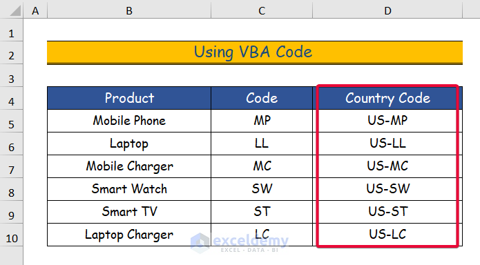
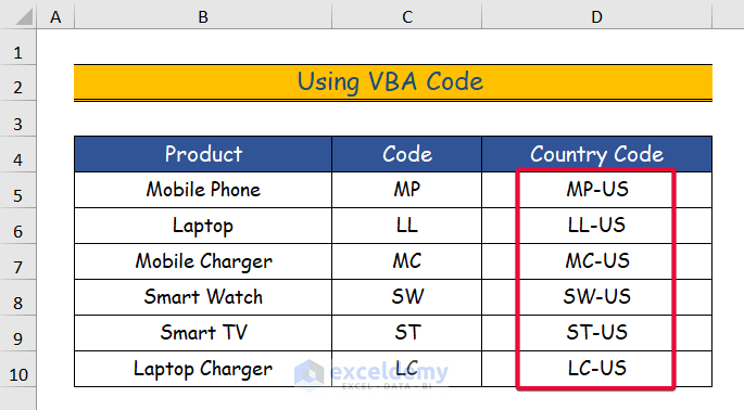
Step 6:
The suffix “US-” is added.
Read More: How to Add Text to Cell Value in Excel
Download the Practice Workbook
Related Articles
- How to Add Text to Beginning of Cell in Excel
- How to Add Text Before a Formula in Excel
- How to Add Text in IF Formula in Excel
<< Go Back to Excel Add Text to Cell Value | Concatenate Excel | Learn Excel
Get FREE Advanced Excel Exercises with Solutions!
