Dataset Overview
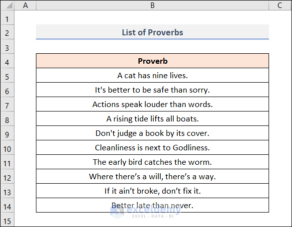
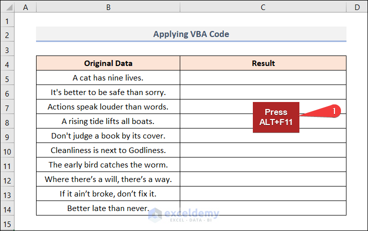
Suppose you have a list of proverbs, which includes ten popular English proverbs. Now, you want to add text to these proverbs. In most cases, you’ll add the prefix Proverb: at the beginning of each text string in the B5:B14 range.
Method 1 – Using Flash Fill Feature
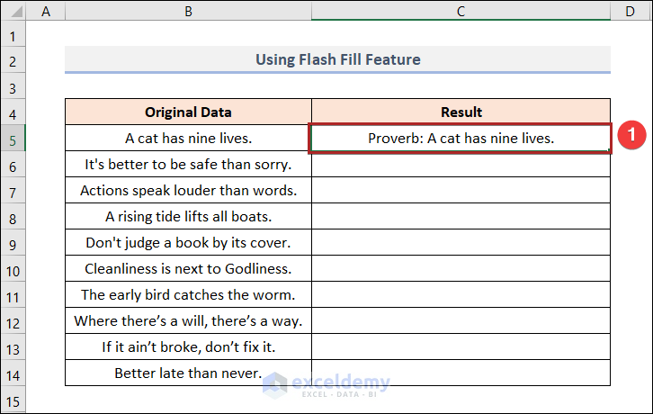
- Start by selecting cell C5.
- Manually type Proverb: A cat has nine lives into that cell.
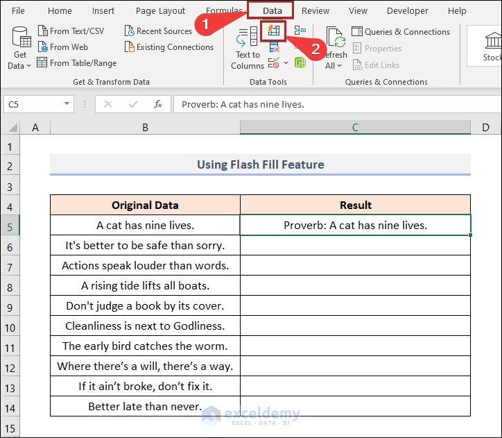
- Go to the Data tab.
- In the Data Tools group, select the Flash Fill feature. Alternatively, you can use the keyboard shortcut CTRL+E.
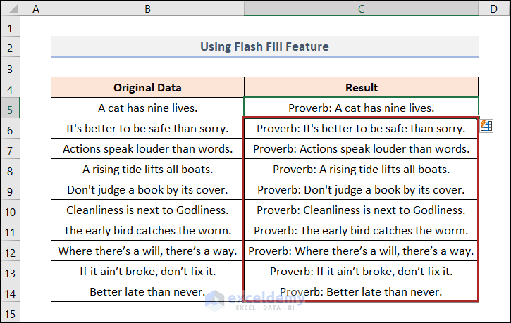
- All the remaining cells in Column C get filled based on the pattern of cell C5.
Read More: How to Add Text to Beginning of Cell in Excel
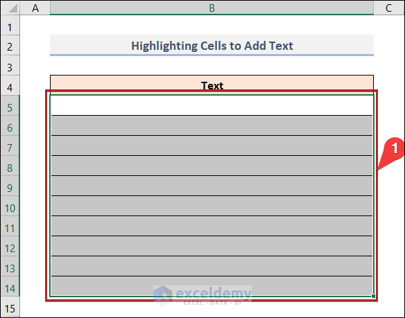
Method 2 – Highlighting Cells to Add Text
- Select the cells in the B5:B14 range. They will become highlighted.
- Manually type the text A cat has nine lives into cell B5.
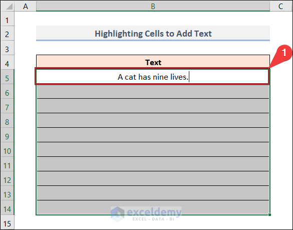
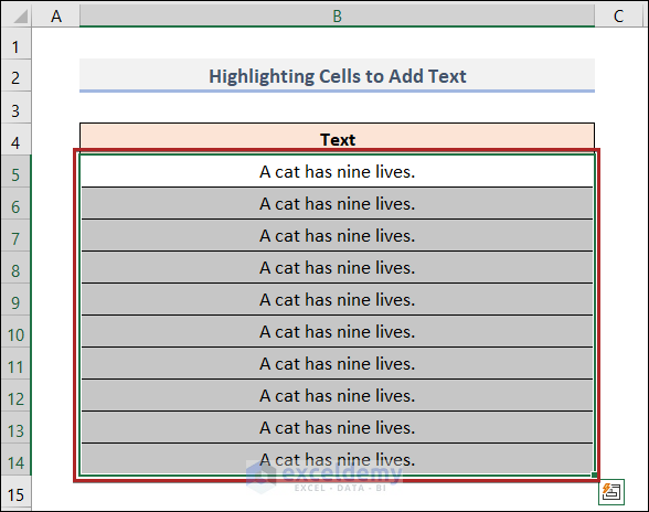
- Press CTRL+ENTER to apply the same text to all the selected cells.
- All the cells will be filled with the same text string.
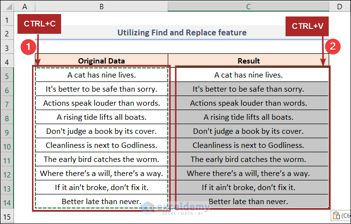
Method 3 – Using the Find and Replace Feature
The fundamental concept behind this technique is to substitute new text for the original text found in the cells. To achieve this, we’ll leverage Excel’s Find and Replace feature. Follow the steps below:
- Select the cells in the B5:B14 range.
- Press CTRL+C to copy the selected cells.
- Select cell C5.
- Press CTRL+V to paste the copied cells into the selected range.
- Press the CTRL key followed by the H key on your keyboard.
- The Find and Replace dialog box will appear.
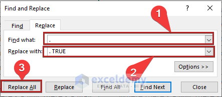
- In the Find what box, enter a full stop ( . ).
- In the Replace with box, type TRUE.
- Click the Replace All button.
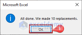
- A warning box may appear; click OK.
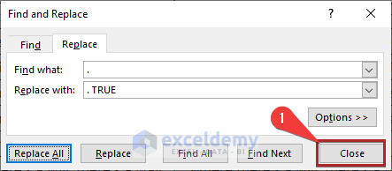
- You’ll be returned to the Find and Replace dialog box.
- Select the Close button.
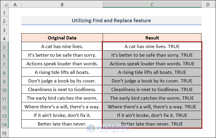
As a result, the text TRUE will be added at the end of the text string in each cell.
Read More: How to Add Text to End of Cell in Excel
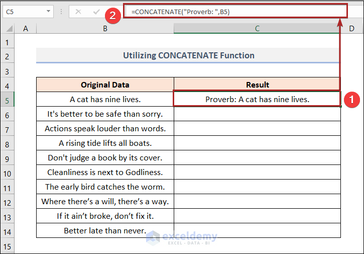
Method 4 – Using the CONCATENATE Function
- Select cell C5.
- In that cell, enter the following formula:
=CONCATENATE("Proverb: ",B5)
Here, B5 represents the cell reference for the first proverb in the Original Data column.
- Press ENTER to apply the formula.
- Move the cursor to the bottom-right corner of cell C5 to see a plus (+) sign (known as the Fill Handle tool).
- Drag the Fill Handle tool down to cell C14 to populate the other results.
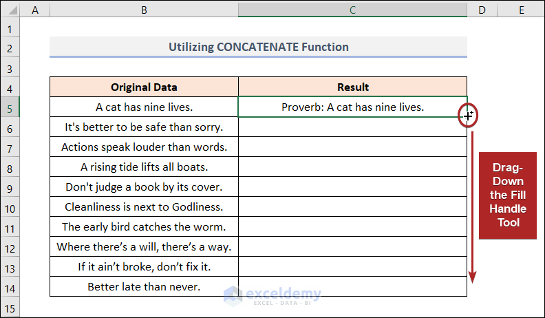
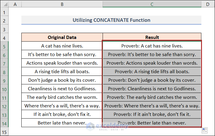
- By doing this, you’ll successfully copy the formula to the remaining cells, resulting in the desired output.
- Your CONCATENATE worksheet should now resemble the one below:
Read More: How to Add a Word in All Rows in Excel
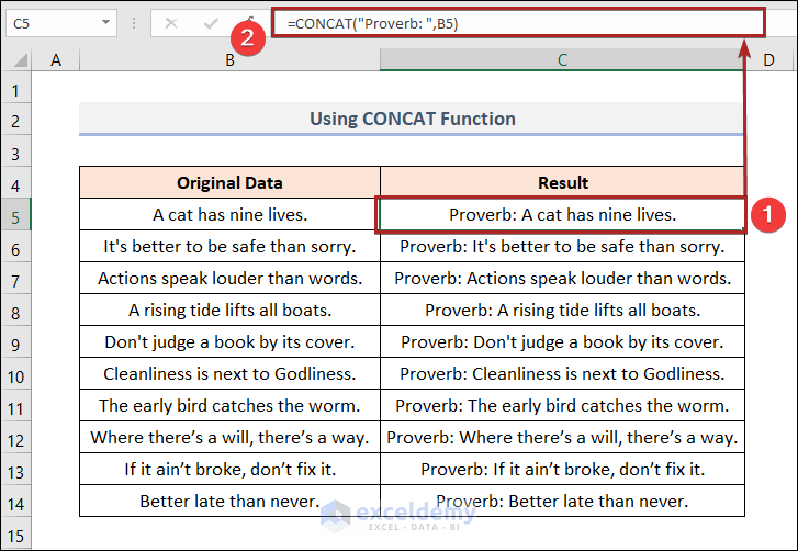
Method 5 – Using the CONCAT Function
In this method, we’ll utilize a modernized replacement for the CONCATENATE function called CONCAT. This function is available in Excel 2019, Excel 365, and Excel Online. If you’re using any of the mentioned versions, you can follow these steps:
- Select cell C5.
- Enter the following formula into cell C5:
=CONCAT("Proverb: ",B5)
Here, B5 represents the cell reference for the 1st proverb in the Original Data column.
- Press the ENTER key to apply the formula.
- Move the cursor to the bottom-right corner of cell C5 to see a plus (+) sign (known as the Fill Handle tool).
- Drag the Fill Handle tool down to cell C14 to populate the other results.
Thus, we can get the other results by using the Fill Handle tool.
Read More: How to Add Text in Excel Spreadsheet
Method 6 – Using the Ampersand Operator to Merge Text Strings
You can easily merge text strings in Excel using the ampersand (&) operator. Here’s how you can use it to add text in multiple cells:
- Select cell C5.
- Enter the following formula:
="Proverb: "&B5
- Press the ENTER key.
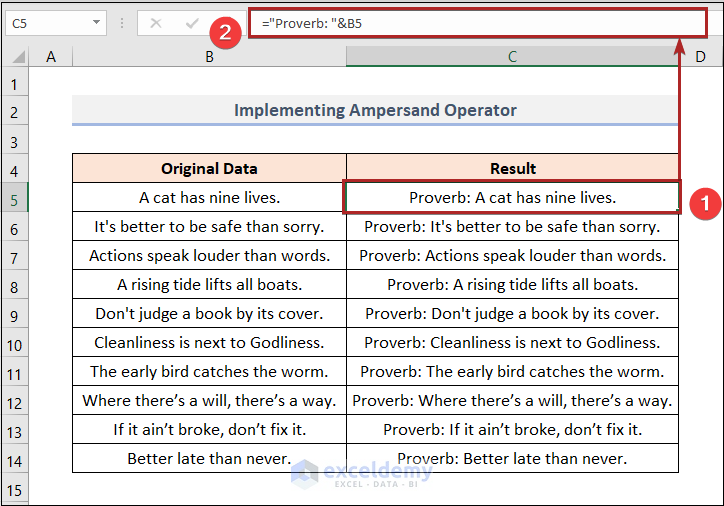
By following these steps, you’ll concatenate the text Proverb: with the content of cell B5. The result will be displayed in cell C5.
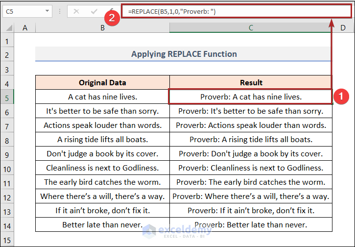
Method 7 – Using the REPLACE Function
- Select cell C5.
- Enter the following formula:
=REPLACE(B5,1,0,"Proverb: ")
-
- The REPLACE function is used to replace a part of a text string with a different text string.
- Its syntax is: REPLACE(old_text, start_num, num_chars, new_text).
- In this case:
- old_text refers to the existing text within which a part needs to be replaced (in cell B5, which contains A cat has nine lives).
- start_num specifies the starting position of the character to be replaced (here, it’s the first character, which is A).
- num_chars indicates the number of characters to replace (since it’s 0, nothing will be replaced; instead, something will be added at the beginning).
- “Proverb: ” is the new text to be added by replacing the old one.
- Press ENTER.
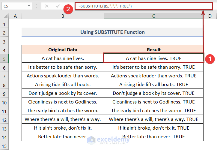
Method 8 – Using the SUBSTITUTE Function
- Select cell C5.
- Enter the following formula:
=SUBSTITUTE(B5,".",". TRUE")
-
- The SUBSTITUDE function replaces specific text within a text string with new text.
- Its syntax is: SUBSTITUDE(text, old_text, new_text).
- In this case:
- text refers to the existing text within which a part needs to be replaced (in cell B5, which contains A cat has nine lives).
- old_text specifies the text to be replaced (here, it’s the period “.”).
- new_text indicates the text to be added by replacing the old one (in this case, “. TRUE”).
- Press ENTER.
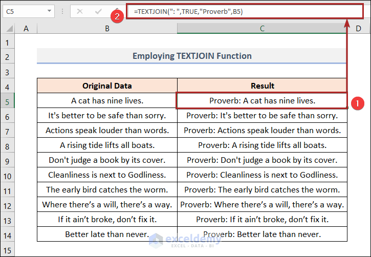
Method 9 – Using the TEXTJOIN Function
- Select cell C5.
- Enter the following formula:
=TEXTJOIN(": ",TRUE,"Proverb",B5)
-
- The TEXTJOIN function returns a text string by joining all the specified texts separated by a delimiter.
- Its syntax is: TEXTJOIN(delimiter,ignore_empty,text1,…).
- In this case:
- delimiter is “: “, which serves as the separator between concatenated texts (note the blank space after the colon).
- ignore_empty is set to TRUE, meaning empty cells will be ignored.
- “Proverb” is the first text string to be joined.
- B5 is the second text string to be joined (in this case, it is A cat has nine lives).
- Press ENTER.
By following these steps, you’ll create a new text string in cell C5 that combines Proverb with the content of cell B5, separated by a colon and space. The result will be displayed in cell C5.
Method 10 – Using VBA Code to Add Text to Multiple Cells
- Press the ALT+F11 key.
- This opens the Microsoft Visual Basic for Applications window.
- Go to the Insert tab.
- Select Module from the options.
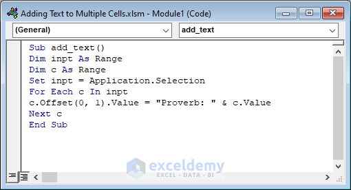
- This opens the code module where you’ll paste the code below:
Sub add_text()
Dim inpt As Range
Dim c As Range
Set inpt = Application.Selection
For Each c In inpt
c.Offset(0, 1).Value = "Proverb: " & c.Value
Next c
End Sub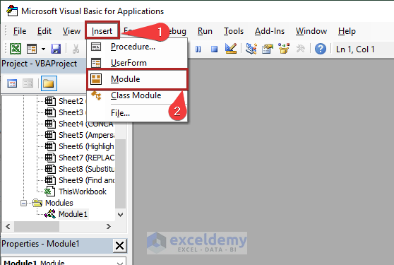
- Save the file as an Excel Macro-enabled workbook.
Code Breakdown:
- Sub add_text(): The lines of code are placed within this subroutine. You can use it anywhere throughout your program.
- Dim inpt As Range and Dim c As Range are variables.
- Set inpt = Application.Selection: When you select a range of cells, they are set as the inpt variable.
- For Each c In inpt: The following operations apply to each cell in the inpt variable.
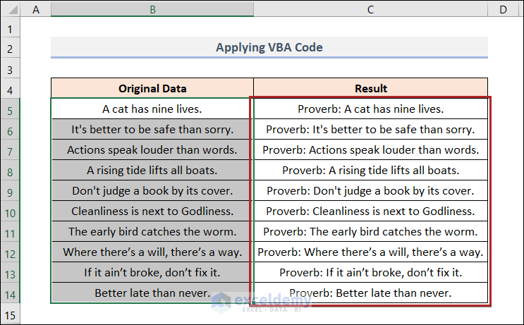
- c.Offset(0, 1).Value = “Proverb: ” & c.Value: By using Offset(0,1), we move one cell to the right (from B5 to C5). The value in cell C5 will be the value of cell B5 concatenated with “Proverb: “ at the beginning.
- Next c: This authorizes the application of the same formula in the next cell within the inpt range.
- End Sub: Indicates the end of the macro.
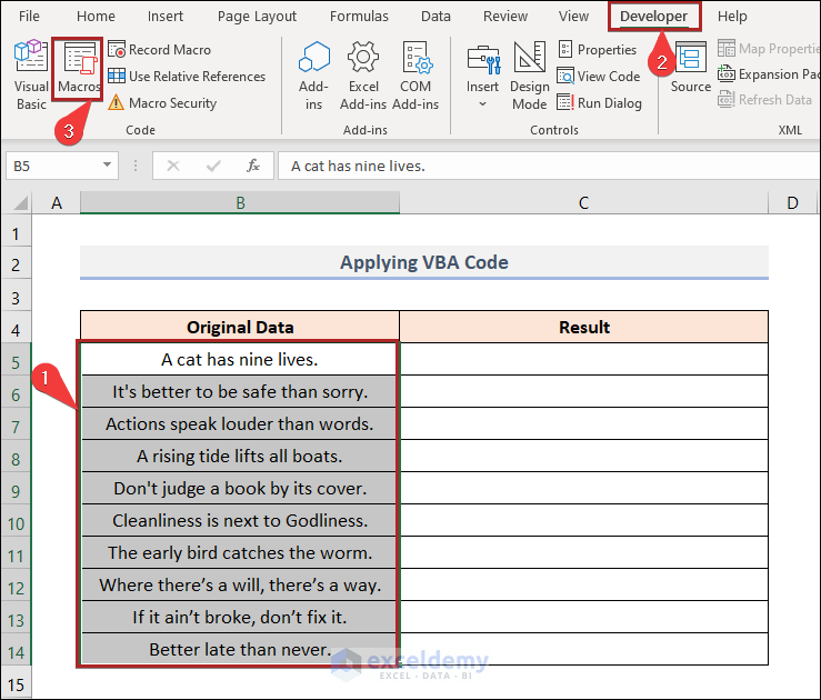
- Return to the worksheet VBA.
- Select cells in the B5:B14 range.
- Go to the Developer tab.
- Select Macros in the Code group.
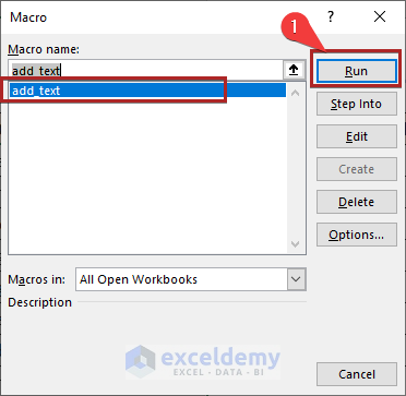
- This opens the Macro dialog box.
- Find the macro named “add_text” (which we’ve just created).
- Click the Run button.
Read More: How to Add Text to Cell Value in Excel
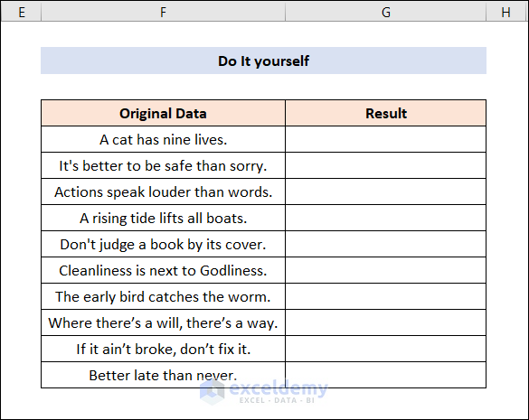
Practice Section
Practice on your own using the Practice section provided on the right side of each sheet.
Download Practice Workbook
You can download the practice workbook from here:
Related Articles
- How to Add Text to Cell Without Deleting in Excel
- How to Add Text in the Middle of a Cell in Excel
- How to Add Text Before a Formula in Excel
- How to Add Text in IF Formula in Excel
- Add Text and Formula in the Same Cell in Excel
<< Go Back to Excel Add Text to Cell Value | Concatenate Excel | Learn Excel
Get FREE Advanced Excel Exercises with Solutions!

