While working with a large Excel worksheet, you may need to freeze the top row and first column. It will allow you to navigate through your entire worksheet keeping the top row and first column always visible. In this article, I’ll show you 5 easy ways to freeze the top row and first column in Excel.
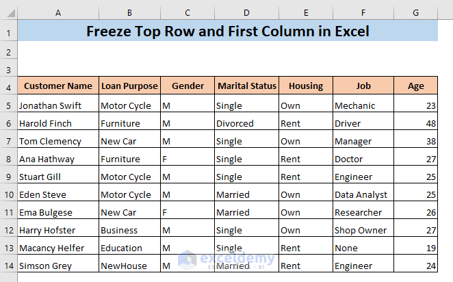
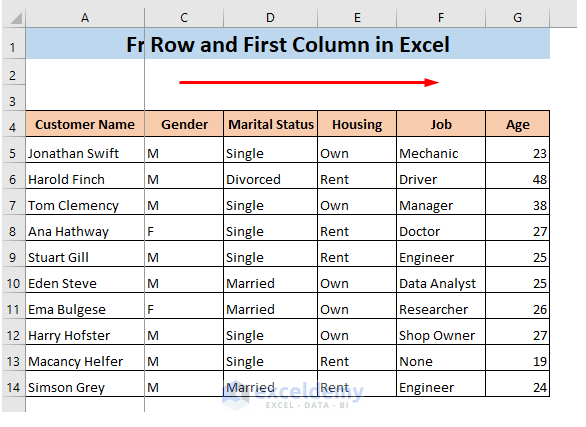
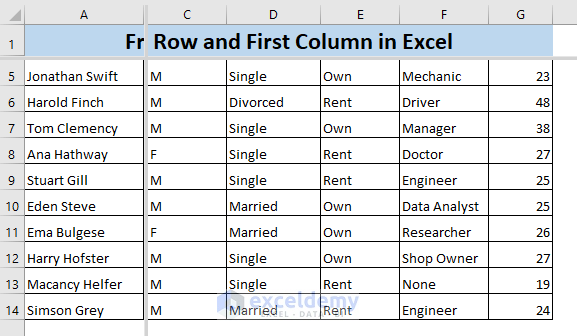
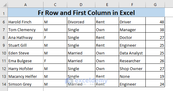
Suppose, you have the following dataset regarding customers’ information, where you want to freeze the top row and the first column.
1. Freezing Excel Top Row Only
To freeze the top row,
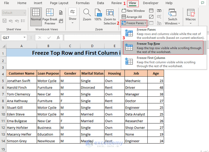
➤ Go to the View tab and click on Freeze Panes from the Window ribbon.
As a result, the Freeze Panes menu will appear.
➤ Click on the Freeze Top Row.
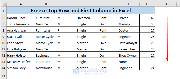
It will freeze the top row of the worksheet. So, if you scroll down, you will see the top row will always remain visible.
Read More: How to Freeze Rows and Columns at the Same Time in Excel
2. Freezing Excel First Column Only
To freeze the first column,
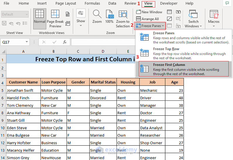
➤ Go to the View tab and click on Freeze Panes from the Window ribbon.
As a result, the Freeze Panes menu will appear.
➤ Click on the Freeze First Column.
It will freeze the first column of the worksheet. So, if you scroll right, you will see the first column will always remain visible.
Read More: Keyboard Shortcut to Freeze Panes in Excel
3. Freezing Top Row and First Column Simultaneously in Excel
In earlier sections, we’ve seen freezing the top row and the first column differently. We can freeze them both simultaneously. Let’s see how to do that. To freeze the top row and first column at the same time,
➤ Select cell B2
The reference cell must be below the row and to the right of the column, you want to freeze. So to freeze the top row and the first column, you need to select cell B2 as the reference cell.
➤ Go to the View tab and click on Freeze Panes from the Window ribbon.
As a result, the Freeze Panes menu will appear.
➤ Click on the Freeze Panes.
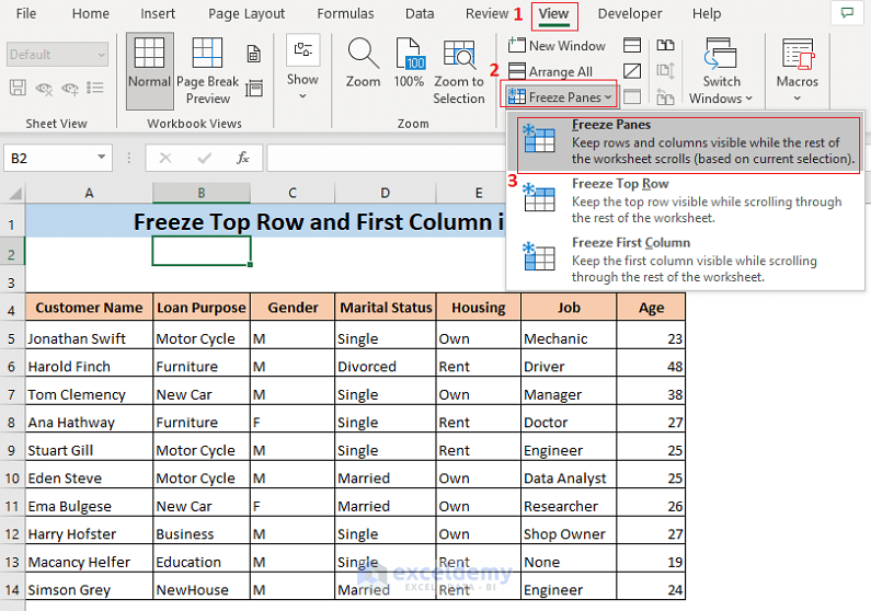
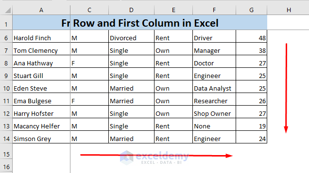
It will freeze both the top row and the first column of the worksheet. So, if you navigate through your worksheet, you will see the top row, and the first column will always remain visible.
4. Splitting Panes to Freeze Top Row and First Column in Excel
Excel offers different features to perform the same task. Freezing is not the exception either. You can also use Split Panes to freeze the top row and the first column of your datasheet.
First,
➤ Select the cell B2
The reference cell must be below the row and to the right of the column, you want to freeze. So to freeze the top row and the first column, you need to select cell B2 as the reference cell.
After that,
➤ Go to the View tab and click on the Split icon.
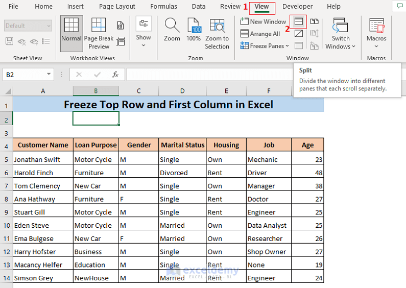
As a result, the top row and the first column of your dataset will be frozen. You will always see the top row and the first column of the sheet regardless of how far you go in the worksheet.
Read More: How to Freeze Multiple Panes in Excel
5. Using Excel Freeze Pane Button to Fix Top Row and First Column
If you frequently need to freeze rows and columns, you can enable a Magic Freeze Button. With this button, you can freeze the top row and the first column very easily. First, let’s see how to create this magic freeze button.
➤ Click on the drop-down icon from the top bar of the Excel files.
It will open a drop-down menu.
➤ Select More Commands from this menu.
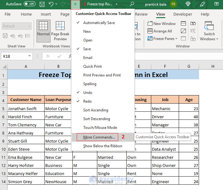
As a result, the Quick Access Toolbar tab of the Excel Options window will appear.
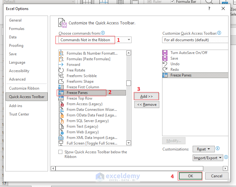
➤ Select Choose Not in the Ribbon in the Choose Command from box.
After that,
➤ Select Freeze Panes and click on Add.
It will add the Freeze Panes option in the right box.
Finally,
➤ Click on OK.
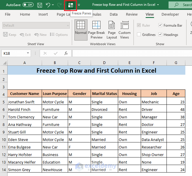
Now, you will see a Freeze Panes icon in the top bar of your Excel file.
To freeze the top row and first column with this magic button,
➤ Select cell B2 and click on this Freeze Panes icon.
It will freeze the top row and the first column of your worksheet.
Read More: How to Apply Custom Freeze Panes in Excel
Things to Remember
🔻 Freeze and split panes cannot be used at the same time. Only one of the two options is available.
🔻 If you want to freeze rows and columns at the same time, the reference cell must be below the row and to the right of the column, you want to freeze. So, to freeze the top row and the first column, you need to select cell B2 as the reference cell.
Download Practice Workbook
Conclusion
I hope now you know how to freeze the top row and first column in Excel. If you want to unfreeze them, you can find the way from here. If you have any kind of confusion, please leave a comment.
Related Articles
- How to Unfreeze Rows and Columns in Excel
- Excel Freeze Panes Not Working
- How to Freeze Panes with VBA in Excel
<< Go Back to Freeze Panes | Learn Excel
Get FREE Advanced Excel Exercises with Solutions!
